Strategies

You can initilize a strategy by R language.

The main libraries are

Quantmod (doc), for loading data and managing the strategy
QuantStrat, for managing the strategy
PerformanceAnalytics, for performance and risk analysis

How to load indicators on your strategy

[1]:

#install.packages("quantmod")
#require(devtools)
#devtools::install_github("braverock/blotter")
#devtools::install_github("braverock/quantstrat")

[2]:

library(quantmod)
# initialization
Sys.setenv(TZ="UTC")
symbol = as.character("AMZN")
start <- as.Date("2017-01-01")
end <- as.Date("2020-01-01")
getSymbols(Symbols = symbol, src = "yahoo", from = start, to = end)

Loading required package: xts

Loading required package: zoo


Attaching package: ‘zoo’


The following objects are masked from ‘package:base’:

    as.Date, as.Date.numeric


Loading required package: TTR

Registered S3 method overwritten by 'quantmod':
  method            from
  as.zoo.data.frame zoo

‘getSymbols’ currently uses auto.assign=TRUE by default, but will
use auto.assign=FALSE in 0.5-0. You will still be able to use
‘loadSymbols’ to automatically load data. getOption("getSymbols.env")
and getOption("getSymbols.auto.assign") will still be checked for
alternate defaults.

This message is shown once per session and may be disabled by setting
options("getSymbols.warning4.0"=FALSE). See ?getSymbols for details.

'AMZN'

[3]:

AMZN <- na.omit(lag(AMZN))
# calculate indicators
sma20 <- SMA(Cl(AMZN), n = 20)
ema20 <- EMA(Cl(AMZN), n = 20)

[4]:

library(quantstrat)
# strategy initialization
currency("USD")
stock(symbol, currency = 'USD', multiplier = 1)
tradeSize <- 100000
initEquity <- 100000
account.st <- portfolio.st <- strategy.st <- "my strategy"
rm.strat("my strategy")
out <- initPortf(portfolio.st, symbols = symbol, initDate = start, currency = "USD")
out <- initAcct(account.st, portfolios = portfolio.st, initDate = start, currency = "USD", initEq = initEquity)
initOrders(portfolio.st, initDate = start)
strategy(strategy.st, store = TRUE)

Loading required package: blotter

Loading required package: FinancialInstrument

Loading required package: PerformanceAnalytics


Attaching package: ‘PerformanceAnalytics’


The following object is masked from ‘package:graphics’:

    legend


Loading required package: foreach

'USD'

'AMZN'

[5]:

# indicators with QuantStrat
out <- add.indicator(strategy.st, name = "SMA", arguments = list(x = quote(Cl(AMZN)), n = 20, maType = "SMA"), label = "SMA20periods")
out <- add.indicator(strategy.st, name = "SMA", arguments = list(x = quote(Cl(AMZN)), n = 50, maType = "SMA"), label = "SMA50periods")
out <- add.indicator(strategy.st, name = "EMA", arguments = list(x = quote(Cl(AMZN)), n = 20, maType = "EMA"), label = "EMA20periods")
out <- add.indicator(strategy.st, name = "EMA", arguments = list(x = quote(Cl(AMZN)), n = 50, maType = "EMA"), label = "EMA50periods")
out <- add.indicator(strategy.st, name = "RSI", arguments = list(price = quote(Cl(AMZN)), n = 7), label = "RSI720periods")
out <- add.indicator(strategy.st, name = "BBands", arguments = list(HLC = quote(Cl(AMZN)), n = 20, maType = "SMA", sd = 2), label = "Bollinger Bands")

[6]:

# custom indicator
RSIaverage <- function(price, n1, n2) {
    RSI_1 <- RSI(price = price, n = n1)
    RSI_2 <- RSI(price = price, n = n2)
    calculatedAverage <- (RSI_1 + RSI_2) / 2
    colnames(calculatedAverage) <- "RSI_average"
    return(calculatedAverage)
}
out <- add.indicator(strategy.st, name = "RSIaverage", arguments = list(price = quote(Cl(AMZN)), n1 = 7, n2 = 14), label = "RSIaverage")

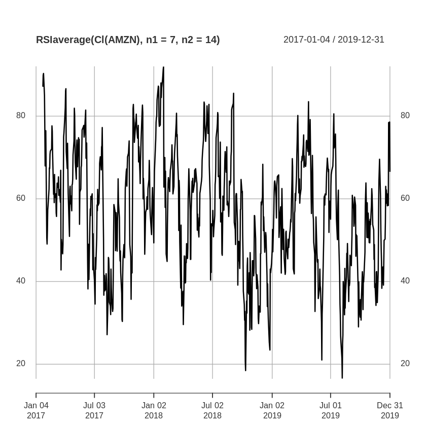
[7]:

# first tests
plot(RSIaverage(Cl(AMZN), n1=7, n2=14)) # for graphing your function results

[8]:

# load all indicators on my data
test <- applyIndicators(strategy = strategy.st, mktdata = OHLC(AMZN))
subsetTest <- test["2018-01-01/2019-01-01"]
head(subsetTest)

           AMZN.Open AMZN.High AMZN.Low AMZN.Close SMA.SMA20periods
2018-01-02   1182.35   1184.00  1167.50    1169.47         1168.841
2018-01-03   1172.00   1190.00  1170.51    1189.01         1170.174
2018-01-04   1188.30   1205.49  1188.30    1204.20         1173.687
2018-01-05   1205.00   1215.87  1204.66    1209.59         1177.088
2018-01-08   1217.51   1229.14  1210.00    1229.14         1180.927
2018-01-09   1236.00   1253.08  1232.03    1246.87         1185.281
           SMA.SMA50periods EMA.EMA20periods EMA.EMA50periods rsi.RSI720periods
2018-01-02         1129.739         1168.779         1130.025          44.92805
2018-01-03         1133.787         1170.706         1132.338          60.65982
2018-01-04         1138.213         1173.896         1135.156          68.75469
2018-01-05         1143.078         1177.295         1138.075          71.20734
2018-01-08         1148.143         1182.233         1141.646          78.38659
2018-01-09         1153.622         1188.389         1145.773          82.89832
           dn.Bollinger.Bands mavg.Bollinger.Bands up.Bollinger.Bands
2018-01-02           1140.397             1168.841           1197.286
2018-01-03           1140.596             1170.174           1199.753
2018-01-04           1145.498             1173.687           1201.876
2018-01-05           1148.806             1177.088           1205.370
2018-01-08           1146.863             1180.927           1214.992
2018-01-09           1142.097             1185.281           1228.466
           pctB.Bollinger.Bands RSI_average.RSIaverage
2018-01-02            0.5110476               49.34830
2018-01-03            0.8183989               60.54486
2018-01-04            1.0412143               66.72199
2018-01-05            1.0746036               68.64585
2018-01-08            1.2076629               74.50261
2018-01-09            1.2130873               78.45513

How to load signals on your strategy

The best practice is to prepare one column for each signal that you want to use on your strategy. The strategy below use the moving averages that they are SMA and EMA. You can use one or the other.

Disclaimer

The strategies below are some simple samples for having an idea how to use the libraries: those strategies are for the educational purpose only. All investments and trading in the stock market involve risk: any decisions related to buying/selling of stocks or other financial instruments should only be made after a thorough research, backtesting, running in demo and seeking a professional assistance if required.

Moving Average Crossover Strategy - Sample 1

when the price value crosses the MA value from below, it will close any existing short position and go long (buy) one unit of the asset
when the price value crosses the MA value from above, it will close any existing long position and go short (sell) one unit of the asset

Reference: https://www.learndatasci.com/tutorials/python-finance-part-3-moving-average-trading-strategy/

[9]:

# Moving Average Crossover Strategy - Sample 1
signalPosition <- function(price, ma) {
    # Taking the difference between the prices and the MA timeseries
    price_ma_diff <- price - ma
    price_ma_diff[is.na(price_ma_diff)] <- 0 # replace missing signals with no position
    # Taking the sign of the difference to determine whether the price or the MA is greater
    position <- diff(price_ma_diff)
    position[is.na(position)] <- 0 # replace missing signals with no position
    colnames(position) <- "Signal_position"
    return(position)
}

[10]:

#out <- add.indicator(strategy.st, name = "signalPosition", arguments = list(price = Cl(AMZN), ma = sma20), label = "signalPosition")
out <- add.indicator(strategy.st, name = "signalPosition", arguments = list(price = Cl(AMZN), ma = ema20), label = "signalPosition1")
out <- add.signal(strategy.st, name = "sigThreshold", arguments = list(column = "Signal_position", threshold = 2, relationship = "gte", cross = TRUE), label = "buy1")
out <- add.signal(strategy.st, name = "sigThreshold", arguments = list(column = "Signal_position", threshold = -2, relationship = "lte", cross = TRUE), label = "sell1")
#add.signal(strategy.st, name = "sigThreshold", arguments = list(data = position, column = "AMZN.Close", threshold = 2, relationship = "gte", cross = TRUE), label = "buy1")
#add.signal(strategy.st, name = "sigThreshold", arguments = list(data = position, column = "AMZN.Close", threshold = -2, relationship = "lte", cross = TRUE), label = "sell1")
# Creating rules
out <- add.rule(strategy.st, name = 'ruleSignal', arguments = list(sigcol = "buy1", sigval = TRUE, orderqty = 100, ordertype = 'market', orderside = 'long'), type = 'enter')
out <- add.rule(strategy.st, name = 'ruleSignal', arguments = list(sigcol = "sell1", sigval = TRUE, orderqty = 'all', ordertype = 'market', orderside = 'long'), type = 'exit')
#out <- add.rule(strategy.st, name = 'ruleSignal', arguments = list(sigcol = "sell1", sigval = TRUE, orderqty = -100, ordertype = 'market', orderside = 'short'), type = 'enter')
#out <- add.rule(strategy.st, name = 'ruleSignal', arguments = list(sigcol = "buy1", sigval = TRUE, orderqty = 'all', ordertype = 'market', orderside = 'short'), type = 'exit')

[11]:

# backtesting
applyStrategy(strategy.st, portfolios=portfolio.st)
out <- updatePortf(portfolio.st)
dateRange <- time(getPortfolio(portfolio.st)$summary)[-1]
out <- updateAcct(portfolio.st, dateRange)
out <- updateEndEq(account.st)
chart.Posn(portfolio.st, Symbol=symbol, TA=c("add_SMA(n=20,col='red')"))

[1] "2017-02-02 00:00:00 AMZN 100 @ 832.349976"
[1] "2017-02-07 00:00:00 AMZN -100 @ 807.640015"
[1] "2017-02-09 00:00:00 AMZN 100 @ 819.710022"
[1] "2017-02-14 00:00:00 AMZN 100 @ 836.530029"
[1] "2017-02-17 00:00:00 AMZN 100 @ 844.140015"
[1] "2017-02-23 00:00:00 AMZN 100 @ 855.609985"
[1] "2017-02-24 00:00:00 AMZN -400 @ 852.190002"
[1] "2017-03-01 00:00:00 AMZN 100 @ 845.039978"
[1] "2017-03-02 00:00:00 AMZN -100 @ 853.080017"
[1] "2017-03-03 00:00:00 AMZN 100 @ 848.909973"
[1] "2017-03-06 00:00:00 AMZN -100 @ 849.880005"
[1] "2017-03-10 00:00:00 AMZN 100 @ 853"
[1] "2017-03-16 00:00:00 AMZN -100 @ 852.969971"
[1] "2017-03-22 00:00:00 AMZN 100 @ 843.200012"
[1] "2017-03-23 00:00:00 AMZN -100 @ 848.059998"
[1] "2017-03-24 00:00:00 AMZN 100 @ 847.380005"
[1] "2017-03-30 00:00:00 AMZN 100 @ 874.320007"
[1] "2017-04-04 00:00:00 AMZN 100 @ 891.51001"
[1] "2017-04-06 00:00:00 AMZN 100 @ 909.280029"
[1] "2017-04-10 00:00:00 AMZN -400 @ 894.880005"
[1] "2017-04-12 00:00:00 AMZN 100 @ 902.359985"
[1] "2017-04-13 00:00:00 AMZN -100 @ 896.22998"
[1] "2017-04-19 00:00:00 AMZN 100 @ 903.780029"
[1] "2017-04-21 00:00:00 AMZN -100 @ 902.059998"
[1] "2017-04-26 00:00:00 AMZN 100 @ 907.619995"
[1] "2017-05-01 00:00:00 AMZN 100 @ 924.98999"
[1] "2017-05-04 00:00:00 AMZN -200 @ 941.030029"
[1] "2017-05-10 00:00:00 AMZN 100 @ 952.820007"
[1] "2017-05-12 00:00:00 AMZN -100 @ 947.619995"
[1] "2017-05-16 00:00:00 AMZN 100 @ 957.969971"
[1] "2017-05-17 00:00:00 AMZN -100 @ 966.070007"
[1] "2017-05-18 00:00:00 AMZN 100 @ 944.76001"
[1] "2017-05-19 00:00:00 AMZN -100 @ 958.48999"
[1] "2017-05-22 00:00:00 AMZN 100 @ 959.840027"
[1] "2017-05-24 00:00:00 AMZN 100 @ 971.539978"
[1] "2017-05-26 00:00:00 AMZN 100 @ 993.380005"
[1] "2017-06-01 00:00:00 AMZN -300 @ 994.619995"
[1] "2017-06-06 00:00:00 AMZN 100 @ 1011.340027"
[1] "2017-06-08 00:00:00 AMZN -100 @ 1010.070007"
[1] "2017-06-09 00:00:00 AMZN 100 @ 1010.27002"
[1] "2017-06-12 00:00:00 AMZN -100 @ 978.309998"
[1] "2017-06-15 00:00:00 AMZN 100 @ 976.469971"
[1] "2017-06-16 00:00:00 AMZN -100 @ 964.169983"
[1] "2017-06-20 00:00:00 AMZN 100 @ 995.169983"
[1] "2017-06-22 00:00:00 AMZN -100 @ 1002.22998"
[1] "2017-06-23 00:00:00 AMZN 100 @ 1001.299988"
[1] "2017-06-26 00:00:00 AMZN -100 @ 1003.73999"
[1] "2017-06-30 00:00:00 AMZN 100 @ 975.929993"
[1] "2017-07-03 00:00:00 AMZN -100 @ 968"
[1] "2017-07-07 00:00:00 AMZN 100 @ 965.140015"
[1] "2017-07-10 00:00:00 AMZN -100 @ 978.76001"
[1] "2017-07-11 00:00:00 AMZN 100 @ 996.469971"
[1] "2017-07-13 00:00:00 AMZN -100 @ 1006.51001"
[1] "2017-07-14 00:00:00 AMZN 100 @ 1000.630005"
[1] "2017-07-17 00:00:00 AMZN -100 @ 1001.809998"
[1] "2017-07-19 00:00:00 AMZN 100 @ 1024.449951"
[1] "2017-07-25 00:00:00 AMZN -100 @ 1038.949951"
[1] "2017-07-26 00:00:00 AMZN 100 @ 1039.869995"
[1] "2017-07-27 00:00:00 AMZN -100 @ 1052.800049"
[1] "2017-07-28 00:00:00 AMZN 100 @ 1046"
[1] "2017-07-31 00:00:00 AMZN -100 @ 1020.039978"
[1] "2017-08-03 00:00:00 AMZN 100 @ 995.890015"
[1] "2017-08-07 00:00:00 AMZN -100 @ 987.580017"
[1] "2017-08-08 00:00:00 AMZN 100 @ 992.27002"
[1] "2017-08-11 00:00:00 AMZN -100 @ 956.919983"
[1] "2017-08-15 00:00:00 AMZN 100 @ 983.299988"
[1] "2017-08-18 00:00:00 AMZN -100 @ 960.570007"
[1] "2017-08-24 00:00:00 AMZN 100 @ 958"
[1] "2017-08-25 00:00:00 AMZN -100 @ 952.450012"
[1] "2017-08-30 00:00:00 AMZN 100 @ 954.059998"
[1] "2017-09-06 00:00:00 AMZN -100 @ 965.27002"
[1] "2017-09-08 00:00:00 AMZN 100 @ 979.469971"
[1] "2017-09-12 00:00:00 AMZN -100 @ 977.960022"
[1] "2017-09-13 00:00:00 AMZN 100 @ 982.580017"
[1] "2017-09-18 00:00:00 AMZN -100 @ 986.789978"
[1] "2017-09-22 00:00:00 AMZN 100 @ 964.650024"
[1] "2017-09-25 00:00:00 AMZN -100 @ 955.099976"
[1] "2017-09-29 00:00:00 AMZN 100 @ 956.400024"
[1] "2017-10-06 00:00:00 AMZN 100 @ 980.849976"
[1] "2017-10-12 00:00:00 AMZN -200 @ 995"
[1] "2017-10-13 00:00:00 AMZN 100 @ 1000.929993"
[1] "2017-10-20 00:00:00 AMZN -100 @ 986.609985"
[1] "2017-10-26 00:00:00 AMZN 100 @ 972.909973"
[1] "2017-10-27 00:00:00 AMZN -100 @ 972.429993"
[1] "2017-10-31 00:00:00 AMZN 100 @ 1110.849976"
[1] "2017-11-02 00:00:00 AMZN -100 @ 1103.680054"
[1] "2017-11-07 00:00:00 AMZN 100 @ 1120.660034"
[1] "2017-11-09 00:00:00 AMZN -100 @ 1132.880005"
[1] "2017-11-10 00:00:00 AMZN 100 @ 1129.130005"
[1] "2017-11-13 00:00:00 AMZN -100 @ 1125.349976"
[1] "2017-11-16 00:00:00 AMZN 100 @ 1126.689941"
[1] "2017-11-17 00:00:00 AMZN -100 @ 1137.290039"
[1] "2017-11-20 00:00:00 AMZN 100 @ 1129.880005"
[1] "2017-11-21 00:00:00 AMZN -100 @ 1126.310059"
[1] "2017-11-24 00:00:00 AMZN 100 @ 1156.160034"
[1] "2017-11-30 00:00:00 AMZN -100 @ 1161.27002"
[1] "2017-12-04 00:00:00 AMZN 100 @ 1162.349976"
[1] "2017-12-05 00:00:00 AMZN -100 @ 1133.949951"
[1] "2017-12-07 00:00:00 AMZN 100 @ 1152.349976"
[1] "2017-12-13 00:00:00 AMZN 100 @ 1165.079956"
[1] "2017-12-14 00:00:00 AMZN -200 @ 1164.130005"
[1] "2017-12-18 00:00:00 AMZN 100 @ 1179.140015"
[1] "2017-12-21 00:00:00 AMZN -100 @ 1177.619995"
[1] "2017-12-28 00:00:00 AMZN 100 @ 1182.26001"
[1] "2018-01-03 00:00:00 AMZN -100 @ 1189.01001"
[1] "2018-01-04 00:00:00 AMZN 100 @ 1204.199951"
[1] "2018-01-09 00:00:00 AMZN 100 @ 1246.869995"
[1] "2018-01-12 00:00:00 AMZN -200 @ 1276.680054"
[1] "2018-01-16 00:00:00 AMZN 100 @ 1305.199951"
[1] "2018-01-18 00:00:00 AMZN -100 @ 1295"
[1] "2018-01-24 00:00:00 AMZN 100 @ 1362.540039"
[1] "2018-01-26 00:00:00 AMZN -100 @ 1377.949951"
[1] "2018-01-29 00:00:00 AMZN 100 @ 1402.050049"
[1] "2018-02-05 00:00:00 AMZN -100 @ 1429.949951"
[1] "2018-02-06 00:00:00 AMZN 100 @ 1390"
[1] "2018-02-07 00:00:00 AMZN -100 @ 1442.839966"
[1] "2018-02-08 00:00:00 AMZN 100 @ 1416.780029"
[1] "2018-02-09 00:00:00 AMZN -100 @ 1350.5"
[1] "2018-02-14 00:00:00 AMZN 100 @ 1414.51001"
[1] "2018-02-21 00:00:00 AMZN -100 @ 1468.349976"
[1] "2018-02-22 00:00:00 AMZN 100 @ 1482.920044"
[1] "2018-02-26 00:00:00 AMZN -100 @ 1500"
[1] "2018-02-27 00:00:00 AMZN 100 @ 1521.949951"
[1] "2018-03-01 00:00:00 AMZN -100 @ 1512.449951"
[1] "2018-03-06 00:00:00 AMZN 100 @ 1523.609985"
[1] "2018-03-13 00:00:00 AMZN 100 @ 1598.390015"
[1] "2018-03-15 00:00:00 AMZN -200 @ 1591"
[1] "2018-03-22 00:00:00 AMZN 100 @ 1581.859985"
[1] "2018-03-23 00:00:00 AMZN -100 @ 1544.920044"
[1] "2018-03-28 00:00:00 AMZN 100 @ 1497.050049"
[1] "2018-03-29 00:00:00 AMZN -100 @ 1431.420044"
[1] "2018-04-03 00:00:00 AMZN 100 @ 1371.98999"
[1] "2018-04-04 00:00:00 AMZN -100 @ 1392.050049"
[1] "2018-04-05 00:00:00 AMZN 100 @ 1410.569946"
[1] "2018-04-10 00:00:00 AMZN -100 @ 1406.079956"
[1] "2018-04-11 00:00:00 AMZN 100 @ 1436.219971"
[1] "2018-04-13 00:00:00 AMZN -100 @ 1448.5"
[1] "2018-04-16 00:00:00 AMZN 100 @ 1430.790039"
[1] "2018-04-17 00:00:00 AMZN -100 @ 1441.5"
[1] "2018-04-18 00:00:00 AMZN 100 @ 1503.829956"
[1] "2018-04-24 00:00:00 AMZN -100 @ 1517.859985"
[1] "2018-04-27 00:00:00 AMZN 100 @ 1517.959961"
[1] "2018-05-02 00:00:00 AMZN -100 @ 1582.26001"
[1] "2018-05-03 00:00:00 AMZN 100 @ 1569.680054"
[1] "2018-05-04 00:00:00 AMZN -100 @ 1572.079956"
[1] "2018-05-08 00:00:00 AMZN 100 @ 1600.140015"
[1] "2018-05-10 00:00:00 AMZN -100 @ 1608"
[1] "2018-05-11 00:00:00 AMZN 100 @ 1609.079956"
[1] "2018-05-14 00:00:00 AMZN -100 @ 1602.910034"
[1] "2018-05-18 00:00:00 AMZN 100 @ 1581.76001"
[1] "2018-05-21 00:00:00 AMZN -100 @ 1574.369995"
[1] "2018-05-23 00:00:00 AMZN 100 @ 1581.400024"
[1] "2018-05-24 00:00:00 AMZN -100 @ 1601.859985"
[1] "2018-05-25 00:00:00 AMZN 100 @ 1603.069946"
[1] "2018-05-30 00:00:00 AMZN 100 @ 1612.869995"
[1] "2018-06-01 00:00:00 AMZN 100 @ 1629.619995"
[1] "2018-06-05 00:00:00 AMZN 100 @ 1665.27002"
[1] "2018-06-08 00:00:00 AMZN -400 @ 1689.300049"
[1] "2018-06-14 00:00:00 AMZN 100 @ 1704.859985"
[1] "2018-06-18 00:00:00 AMZN 100 @ 1715.969971"
[1] "2018-06-19 00:00:00 AMZN -200 @ 1723.790039"
[1] "2018-06-21 00:00:00 AMZN 100 @ 1750.079956"
[1] "2018-06-25 00:00:00 AMZN -100 @ 1715.670044"
[1] "2018-06-28 00:00:00 AMZN 100 @ 1660.51001"
[1] "2018-06-29 00:00:00 AMZN -100 @ 1701.449951"
[1] "2018-07-02 00:00:00 AMZN 100 @ 1699.800049"
[1] "2018-07-03 00:00:00 AMZN -100 @ 1713.780029"
[1] "2018-07-05 00:00:00 AMZN 100 @ 1693.959961"
[1] "2018-07-06 00:00:00 AMZN -100 @ 1699.72998"
[1] "2018-07-09 00:00:00 AMZN 100 @ 1710.630005"
[1] "2018-07-13 00:00:00 AMZN 100 @ 1796.619995"
[1] "2018-07-19 00:00:00 AMZN 100 @ 1842.920044"
[1] "2018-07-20 00:00:00 AMZN -300 @ 1812.969971"
[1] "2018-07-26 00:00:00 AMZN 100 @ 1863.609985"
[1] "2018-07-30 00:00:00 AMZN -100 @ 1817.27002"
[1] "2018-07-31 00:00:00 AMZN 100 @ 1779.219971"
[1] "2018-08-01 00:00:00 AMZN -100 @ 1777.439941"
[1] "2018-08-03 00:00:00 AMZN 100 @ 1834.329956"
[1] "2018-08-07 00:00:00 AMZN -100 @ 1847.75"
[1] "2018-08-08 00:00:00 AMZN 100 @ 1862.47998"
[1] "2018-08-14 00:00:00 AMZN -100 @ 1896.199951"
[1] "2018-08-15 00:00:00 AMZN 100 @ 1919.650024"
[1] "2018-08-17 00:00:00 AMZN -100 @ 1886.52002"
[1] "2018-08-23 00:00:00 AMZN 100 @ 1904.900024"
[1] "2018-08-27 00:00:00 AMZN -100 @ 1905.390015"
[1] "2018-08-29 00:00:00 AMZN 100 @ 1932.819946"
[1] "2018-08-31 00:00:00 AMZN 100 @ 2002.380005"
[1] "2018-09-04 00:00:00 AMZN -200 @ 2012.709961"
[1] "2018-09-06 00:00:00 AMZN 100 @ 1994.819946"
[1] "2018-09-07 00:00:00 AMZN -100 @ 1958.310059"
[1] "2018-09-13 00:00:00 AMZN 100 @ 1990"
[1] "2018-09-17 00:00:00 AMZN -100 @ 1970.189941"
[1] "2018-09-20 00:00:00 AMZN 100 @ 1926.420044"
[1] "2018-09-21 00:00:00 AMZN -100 @ 1944.300049"
[1] "2018-09-24 00:00:00 AMZN 100 @ 1915.01001"
[1] "2018-09-25 00:00:00 AMZN -100 @ 1934.359985"
[1] "2018-09-26 00:00:00 AMZN 100 @ 1974.550049"
[1] "2018-09-28 00:00:00 AMZN -100 @ 2012.97998"
[1] "2018-10-01 00:00:00 AMZN 100 @ 2003"
[1] "2018-10-02 00:00:00 AMZN -100 @ 2004.359985"
[1] "2018-10-11 00:00:00 AMZN 100 @ 1755.25"
[1] "2018-10-12 00:00:00 AMZN -100 @ 1719.359985"
[1] "2018-10-16 00:00:00 AMZN 100 @ 1760.949951"
[1] "2018-10-17 00:00:00 AMZN -100 @ 1819.959961"
[1] "2018-10-18 00:00:00 AMZN 100 @ 1831.72998"
[1] "2018-10-22 00:00:00 AMZN -100 @ 1764.030029"
[1] "2018-10-23 00:00:00 AMZN 100 @ 1789.300049"
[1] "2018-10-25 00:00:00 AMZN -100 @ 1664.199951"
[1] "2018-10-29 00:00:00 AMZN 100 @ 1642.810059"
[1] "2018-10-30 00:00:00 AMZN -100 @ 1538.880005"
[1] "2018-11-01 00:00:00 AMZN 100 @ 1598.01001"
[1] "2018-11-07 00:00:00 AMZN -100 @ 1642.810059"
[1] "2018-11-08 00:00:00 AMZN 100 @ 1755.48999"
[1] "2018-11-12 00:00:00 AMZN -100 @ 1712.430054"
[1] "2018-11-19 00:00:00 AMZN 100 @ 1593.410034"
[1] "2018-11-20 00:00:00 AMZN -100 @ 1512.290039"
[1] "2018-11-26 00:00:00 AMZN 100 @ 1502.060059"
[1] "2018-11-27 00:00:00 AMZN -100 @ 1581.329956"
[1] "2018-11-28 00:00:00 AMZN 100 @ 1581.420044"
[1] "2018-12-03 00:00:00 AMZN -100 @ 1690.170044"
[1] "2018-12-04 00:00:00 AMZN 100 @ 1772.359985"
[1] "2018-12-07 00:00:00 AMZN -100 @ 1699.189941"
[1] "2018-12-10 00:00:00 AMZN 100 @ 1629.130005"
[1] "2018-12-11 00:00:00 AMZN -100 @ 1641.030029"
[1] "2018-12-12 00:00:00 AMZN 100 @ 1643.23999"
[1] "2018-12-17 00:00:00 AMZN -100 @ 1591.910034"
[1] "2018-12-20 00:00:00 AMZN 100 @ 1495.079956"
[1] "2018-12-21 00:00:00 AMZN -100 @ 1460.829956"
[1] "2018-12-28 00:00:00 AMZN 100 @ 1461.640015"
[1] "2019-01-02 00:00:00 AMZN 100 @ 1501.969971"
[1] "2019-01-07 00:00:00 AMZN -200 @ 1575.390015"
[1] "2019-01-08 00:00:00 AMZN 100 @ 1629.51001"
[1] "2019-01-11 00:00:00 AMZN -100 @ 1656.219971"
[1] "2019-01-17 00:00:00 AMZN 100 @ 1683.780029"
[1] "2019-01-23 00:00:00 AMZN -100 @ 1632.170044"
[1] "2019-01-25 00:00:00 AMZN 100 @ 1654.930054"
[1] "2019-01-30 00:00:00 AMZN -100 @ 1593.880005"
[1] "2019-02-01 00:00:00 AMZN 100 @ 1718.72998"
[1] "2019-02-05 00:00:00 AMZN -100 @ 1633.310059"
[1] "2019-02-06 00:00:00 AMZN 100 @ 1658.810059"
[1] "2019-02-08 00:00:00 AMZN -100 @ 1614.369995"
[1] "2019-02-13 00:00:00 AMZN 100 @ 1638.01001"
[1] "2019-02-19 00:00:00 AMZN -100 @ 1607.949951"
[1] "2019-02-21 00:00:00 AMZN 100 @ 1622.099976"
[1] "2019-02-22 00:00:00 AMZN -100 @ 1619.439941"
[1] "2019-02-26 00:00:00 AMZN 100 @ 1633"
[1] "2019-02-28 00:00:00 AMZN 100 @ 1641.089966"
[1] "2019-03-04 00:00:00 AMZN -200 @ 1671.72998"
[1] "2019-03-05 00:00:00 AMZN 100 @ 1696.170044"
[1] "2019-03-07 00:00:00 AMZN -100 @ 1668.949951"
[1] "2019-03-13 00:00:00 AMZN 100 @ 1673.099976"
[1] "2019-03-15 00:00:00 AMZN 100 @ 1686.219971"
[1] "2019-03-18 00:00:00 AMZN -200 @ 1712.359985"
[1] "2019-03-19 00:00:00 AMZN 100 @ 1742.150024"
[1] "2019-03-26 00:00:00 AMZN -100 @ 1774.26001"
[1] "2019-03-27 00:00:00 AMZN 100 @ 1783.76001"
[1] "2019-03-29 00:00:00 AMZN -100 @ 1773.420044"
[1] "2019-04-01 00:00:00 AMZN 100 @ 1780.75"
[1] "2019-04-04 00:00:00 AMZN -100 @ 1820.699951"
[1] "2019-04-09 00:00:00 AMZN 100 @ 1849.859985"
[1] "2019-04-11 00:00:00 AMZN -100 @ 1847.329956"
[1] "2019-04-12 00:00:00 AMZN 100 @ 1844.069946"
[1] "2019-04-15 00:00:00 AMZN -100 @ 1843.060059"
[1] "2019-04-18 00:00:00 AMZN 100 @ 1864.819946"
[1] "2019-04-22 00:00:00 AMZN -100 @ 1861.689941"
[1] "2019-04-24 00:00:00 AMZN 100 @ 1923.77002"
[1] "2019-04-26 00:00:00 AMZN -100 @ 1902.25"
[1] "2019-04-30 00:00:00 AMZN 100 @ 1938.430054"
[1] "2019-05-01 00:00:00 AMZN -100 @ 1926.52002"
[1] "2019-05-07 00:00:00 AMZN 100 @ 1950.550049"
[1] "2019-05-08 00:00:00 AMZN -100 @ 1921"
[1] "2019-05-16 00:00:00 AMZN 100 @ 1871.150024"
[1] "2019-05-21 00:00:00 AMZN -100 @ 1858.969971"
[1] "2019-05-24 00:00:00 AMZN 100 @ 1815.47998"
[1] "2019-05-28 00:00:00 AMZN -100 @ 1823.280029"
[1] "2019-05-29 00:00:00 AMZN 100 @ 1836.430054"
[1] "2019-05-31 00:00:00 AMZN -100 @ 1816.319946"
[1] "2019-06-06 00:00:00 AMZN 100 @ 1738.5"
[1] "2019-06-14 00:00:00 AMZN -100 @ 1870.300049"
[1] "2019-06-17 00:00:00 AMZN 100 @ 1869.670044"
[1] "2019-06-18 00:00:00 AMZN -100 @ 1886.030029"
[1] "2019-06-19 00:00:00 AMZN 100 @ 1901.369995"
[1] "2019-06-24 00:00:00 AMZN 100 @ 1911.300049"
[1] "2019-06-25 00:00:00 AMZN -200 @ 1913.900024"
[1] "2019-06-28 00:00:00 AMZN 100 @ 1904.280029"
[1] "2019-07-02 00:00:00 AMZN -100 @ 1922.189941"
[1] "2019-07-03 00:00:00 AMZN 100 @ 1934.310059"
[1] "2019-07-10 00:00:00 AMZN 100 @ 1988.300049"
[1] "2019-07-15 00:00:00 AMZN -200 @ 2011"
[1] "2019-07-24 00:00:00 AMZN 100 @ 1994.48999"
[1] "2019-07-29 00:00:00 AMZN -100 @ 1943.050049"
[1] "2019-08-08 00:00:00 AMZN 100 @ 1793.400024"
[1] "2019-08-13 00:00:00 AMZN -100 @ 1784.920044"
[1] "2019-08-15 00:00:00 AMZN 100 @ 1762.959961"
[1] "2019-08-16 00:00:00 AMZN -100 @ 1776.119995"
[1] "2019-08-19 00:00:00 AMZN 100 @ 1792.569946"
[1] "2019-08-22 00:00:00 AMZN -100 @ 1823.540039"
[1] "2019-08-23 00:00:00 AMZN 100 @ 1804.660034"
[1] "2019-08-26 00:00:00 AMZN -100 @ 1749.619995"
[1] "2019-08-28 00:00:00 AMZN 100 @ 1761.829956"
[1] "2019-08-30 00:00:00 AMZN 100 @ 1786.400024"
[1] "2019-09-04 00:00:00 AMZN -200 @ 1789.839966"
[1] "2019-09-05 00:00:00 AMZN 100 @ 1800.619995"
[1] "2019-09-10 00:00:00 AMZN -100 @ 1831.349976"
[1] "2019-09-16 00:00:00 AMZN 100 @ 1839.339966"
[1] "2019-09-17 00:00:00 AMZN -100 @ 1807.839966"
[1] "2019-09-19 00:00:00 AMZN 100 @ 1817.459961"
[1] "2019-09-20 00:00:00 AMZN -100 @ 1821.5"
[1] "2019-09-23 00:00:00 AMZN 100 @ 1794.160034"
[1] "2019-09-24 00:00:00 AMZN -100 @ 1785.300049"
[1] "2019-09-27 00:00:00 AMZN 100 @ 1739.839966"
[1] "2019-09-30 00:00:00 AMZN -100 @ 1725.449951"
[1] "2019-10-02 00:00:00 AMZN 100 @ 1735.650024"
[1] "2019-10-04 00:00:00 AMZN -100 @ 1724.420044"
[1] "2019-10-07 00:00:00 AMZN 100 @ 1739.650024"
[1] "2019-10-09 00:00:00 AMZN -100 @ 1705.51001"
[1] "2019-10-11 00:00:00 AMZN 100 @ 1720.26001"
[1] "2019-10-15 00:00:00 AMZN 100 @ 1736.430054"
[1] "2019-10-22 00:00:00 AMZN -200 @ 1785.660034"
[1] "2019-10-23 00:00:00 AMZN 100 @ 1765.72998"
[1] "2019-10-24 00:00:00 AMZN -100 @ 1762.170044"
[1] "2019-10-28 00:00:00 AMZN 100 @ 1761.329956"
[1] "2019-10-29 00:00:00 AMZN -100 @ 1777.079956"
[1] "2019-10-30 00:00:00 AMZN 100 @ 1762.709961"
[1] "2019-10-31 00:00:00 AMZN -100 @ 1779.98999"
[1] "2019-11-01 00:00:00 AMZN 100 @ 1776.660034"
[1] "2019-11-04 00:00:00 AMZN -100 @ 1791.439941"
[1] "2019-11-05 00:00:00 AMZN 100 @ 1804.660034"
[1] "2019-11-07 00:00:00 AMZN -100 @ 1795.77002"
[1] "2019-11-14 00:00:00 AMZN 100 @ 1753.109985"
[1] "2019-11-15 00:00:00 AMZN -100 @ 1754.599976"
[1] "2019-11-18 00:00:00 AMZN 100 @ 1739.48999"
[1] "2019-11-19 00:00:00 AMZN -100 @ 1752.530029"
[1] "2019-11-20 00:00:00 AMZN 100 @ 1752.790039"
[1] "2019-11-22 00:00:00 AMZN -100 @ 1734.709961"
[1] "2019-11-26 00:00:00 AMZN 100 @ 1773.839966"
[1] "2019-12-03 00:00:00 AMZN -100 @ 1781.599976"
[1] "2019-12-10 00:00:00 AMZN 100 @ 1749.51001"
[1] "2019-12-12 00:00:00 AMZN -100 @ 1748.719971"
[1] "2019-12-13 00:00:00 AMZN 100 @ 1760.329956"
[1] "2019-12-18 00:00:00 AMZN 100 @ 1790.660034"
[1] "2019-12-20 00:00:00 AMZN -200 @ 1792.280029"
[1] "2019-12-23 00:00:00 AMZN 100 @ 1786.5"
[1] "2019-12-24 00:00:00 AMZN -100 @ 1793"
[1] "2019-12-26 00:00:00 AMZN 100 @ 1789.209961"
[1] "2019-12-27 00:00:00 AMZN -100 @ 1868.77002"
[1] "2019-12-30 00:00:00 AMZN 100 @ 1869.800049"
[1] "2019-12-31 00:00:00 AMZN -100 @ 1846.890015"

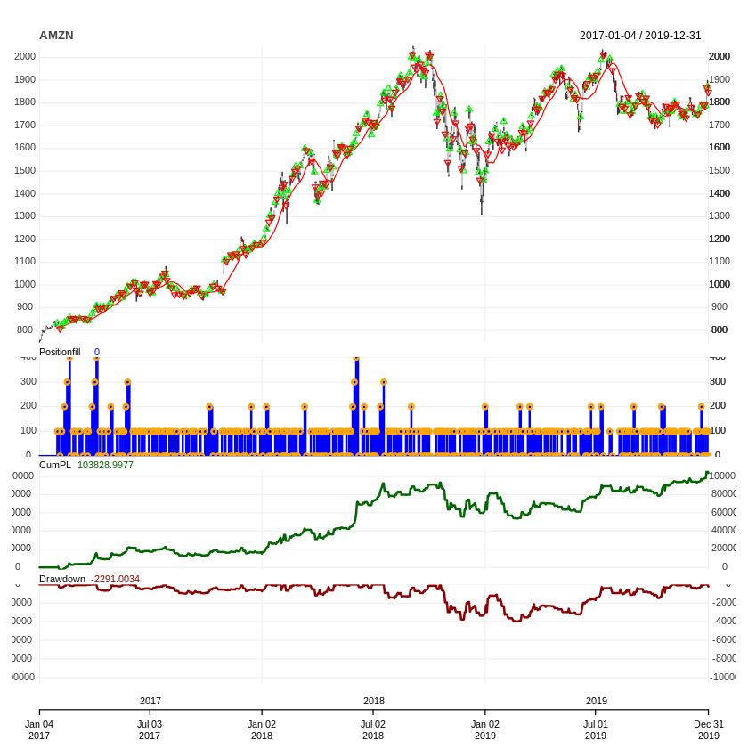
[12]:

tstats <- tradeStats(portfolio.st, use="trades", inclZeroDays=FALSE)
data.frame(t(tstats))

A data.frame: 32 × 1
	AMZN
	<chr>
Portfolio	my strategy
Symbol	AMZN
Num.Txns	348
Num.Trades	160
Net.Trading.PL	103829
Avg.Trade.PL	648.9312
Med.Trade.PL	194.4946
Largest.Winner	24637.02
Largest.Loser	-12510.01
Gross.Profits	297592
Gross.Losses	-193763
Std.Dev.Trade.PL	4650.819
Std.Err.Trade.PL	367.6795
Percent.Positive	53.125
Percent.Negative	46.875
Profit.Factor	1.535856
Avg.Win.Trade	3501.083
Med.Win.Trade	1707.996
Avg.Losing.Trade	-2583.507
Med.Losing.Trade	-1808.008
Avg.Daily.PL	648.9312
Med.Daily.PL	194.4947
Std.Dev.Daily.PL	4650.819
Std.Err.Daily.PL	367.6795
Ann.Sharpe	2.214979
Max.Drawdown	-39630.02
Profit.To.Max.Draw	2.619958
Avg.WinLoss.Ratio	1.355167
Med.WinLoss.Ratio	0.9446838
Max.Equity	106120
Min.Equity	-2470.996
End.Equity	103829

[13]:

#install.packages("magrittr") # package installations are only needed the first time you use it
#install.packages("dplyr")    # alternative installation of the %>%
library(magrittr) # needs to be run every time you start R and want to use %>%
library(dplyr)    # alternatively, this also loads %>%
trades <- tstats %>%
    mutate(Trades = Num.Trades,
        Win.Percent = Percent.Positive,
        Loss.Percent = Percent.Negative,
        WL.Ratio = Percent.Positive/Percent.Negative) %>%
    select(Trades, Win.Percent, Loss.Percent, WL.Ratio)
data.frame(t(trades))


Attaching package: ‘dplyr’


The following objects are masked from ‘package:xts’:

    first, last


The following objects are masked from ‘package:stats’:

    filter, lag


The following objects are masked from ‘package:base’:

    intersect, setdiff, setequal, union

A data.frame: 4 × 1
	t.trades.
	<dbl>
Trades	160.000000
Win.Percent	53.125000
Loss.Percent	46.875000
WL.Ratio	1.133333

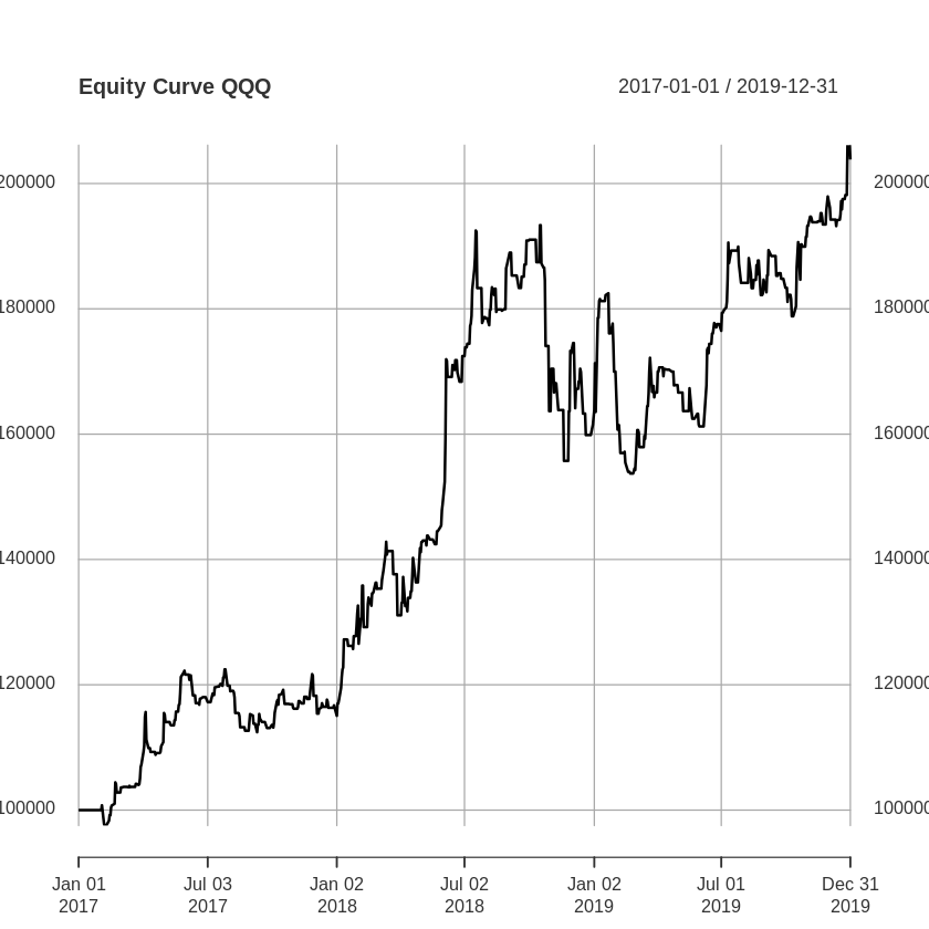
[14]:

a <- getAccount(account.st)
equity <- a$summary$End.Eq
plot(equity, main = "Equity Curve QQQ")

[15]:

portfolio <- getPortfolio(portfolio.st)
portfolioSummary <- portfolio$summary
colnames(portfolio$summary)
tail(portfolio$summary)

'Long.Value'
'Short.Value'
'Net.Value'
'Gross.Value'
'Period.Realized.PL'
'Period.Unrealized.PL'
'Gross.Trading.PL'
'Txn.Fees'
'Net.Trading.PL'

           Long.Value Short.Value Net.Value Gross.Value Period.Realized.PL
2019-12-23     178650           0    178650      178650              0.000
2019-12-24          0           0         0           0            650.000
2019-12-26     178921           0    178921      178921              0.000
2019-12-27          0           0         0           0           7956.006
2019-12-30     186980           0    186980      186980              0.000
2019-12-31          0           0         0           0          -2291.003
           Period.Unrealized.PL Gross.Trading.PL Txn.Fees Net.Trading.PL
2019-12-23                    0            0.000        0          0.000
2019-12-24                    0          650.000        0        650.000
2019-12-26                    0            0.000        0          0.000
2019-12-27                    0         7956.006        0       7956.006
2019-12-30                    0            0.000        0          0.000
2019-12-31                    0        -2291.003        0      -2291.003

[16]:

ret <- Return.calculate(equity, method = "log")
tail(ret)
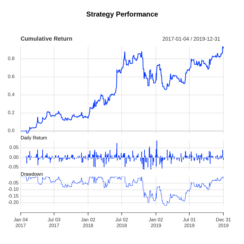
charts.PerformanceSummary(ret, colorset = bluefocus, main = "Strategy Performance")

                 End.Eq
2019-12-23  0.000000000
2019-12-24  0.003285503
2019-12-26  0.000000000
2019-12-27  0.039363582
2019-12-30  0.000000000
2019-12-31 -0.011177133

[17]:

rets <- PortfReturns(Account = account.st)
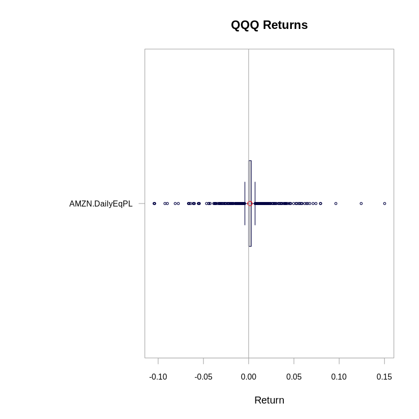
chart.Boxplot(rets, main = "QQQ Returns", colorset= rich10equal)

[18]:

table.Drawdowns(rets, top=10)

A data.frame: 10 × 7
From	Trough	To	Depth	Length	To Trough	Recovery
<date>	<date>	<date>	<dbl>	<dbl>	<dbl>	<dbl>
2018-07-19	2019-02-22	2019-12-27	-0.3726	364	150	214
2018-03-14	2018-03-29	2018-05-10	-0.1135	41	12	29
2017-07-31	2017-09-11	2018-01-12	-0.0966	116	30	86
2017-04-07	2017-04-20	2017-05-23	-0.0671	32	9	23
2018-02-09	2018-02-09	2018-02-26	-0.0663	11	1	10
2018-02-02	2018-02-02	2018-02-07	-0.0609	4	1	3
2017-06-01	2017-06-21	2017-07-27	-0.0535	40	15	25
2018-06-07	2018-06-25	2018-06-29	-0.0362	17	13	4
2017-02-06	2017-02-07	2017-02-21	-0.0322	11	2	9
2019-12-31	2019-12-31	NA	-0.0229	2	1	NA

[19]:

table.CalendarReturns(rets)

A data.frame: 3 × 13
	Jan	Feb	Mar	Apr	May	Jun	Jul	Aug	Sep	Oct	Nov	Dec	AMZN.DailyEqPL
	<dbl>	<dbl>	<dbl>	<dbl>	<dbl>	<dbl>	<dbl>	<dbl>	<dbl>	<dbl>	<dbl>	<dbl>	<dbl>
2017	0	0.0	0.4	0.9	0.3	0.0	-2.6	1.4	0.0	0.0	-3.2	0.4	-2.6
2018	2	-1.0	-6.6	5.5	2.4	4.1	0.0	0.4	3.8	0.0	-0.4	1.6	12.0
2019	0	0.5	0.8	0.0	-0.3	0.0	0.0	2.2	-1.4	1.7	2.2	-2.3	3.3

[20]:

table.DownsideRisk(rets)

A data.frame: 11 × 1
	AMZN.DailyEqPL
	<dbl>
Semi Deviation	0.0143
Gain Deviation	0.0208
Loss Deviation	0.0225
Downside Deviation (MAR=210%)	0.0177
Downside Deviation (Rf=0%)	0.0138
Downside Deviation (0%)	0.0138
Maximum Drawdown	0.3726
Historical VaR (95%)	-0.0277
Historical ES (95%)	-0.0528
Modified VaR (95%)	-0.0264
Modified ES (95%)	-0.0264

[21]:

table.Stats(rets)

A data.frame: 16 × 1
	AMZN.DailyEqPL
	<dbl>
Observations	753.0000
NAs	0.0000
Minimum	-0.1045
Quartile 1	0.0000
Median	0.0000
Arithmetic Mean	0.0014
Geometric Mean	0.0012
Quartile 3	0.0029
Maximum	0.1502
SE Mean	0.0007
LCL Mean (0.95)	-0.0001
UCL Mean (0.95)	0.0028
Variance	0.0004
Stdev	0.0206
Skewness	0.2160
Kurtosis	11.3408

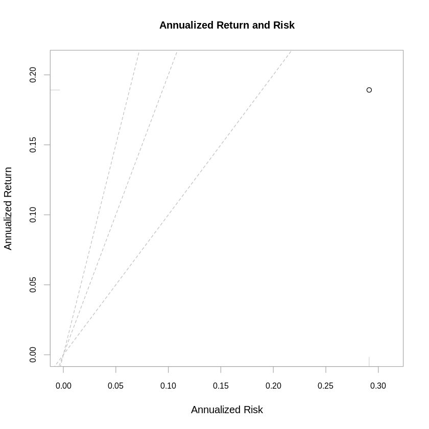
[22]:

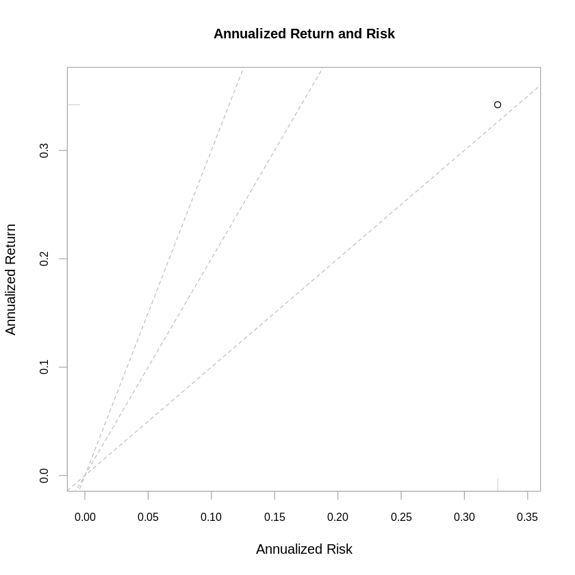
chart.RiskReturnScatter(rets)

[23]:

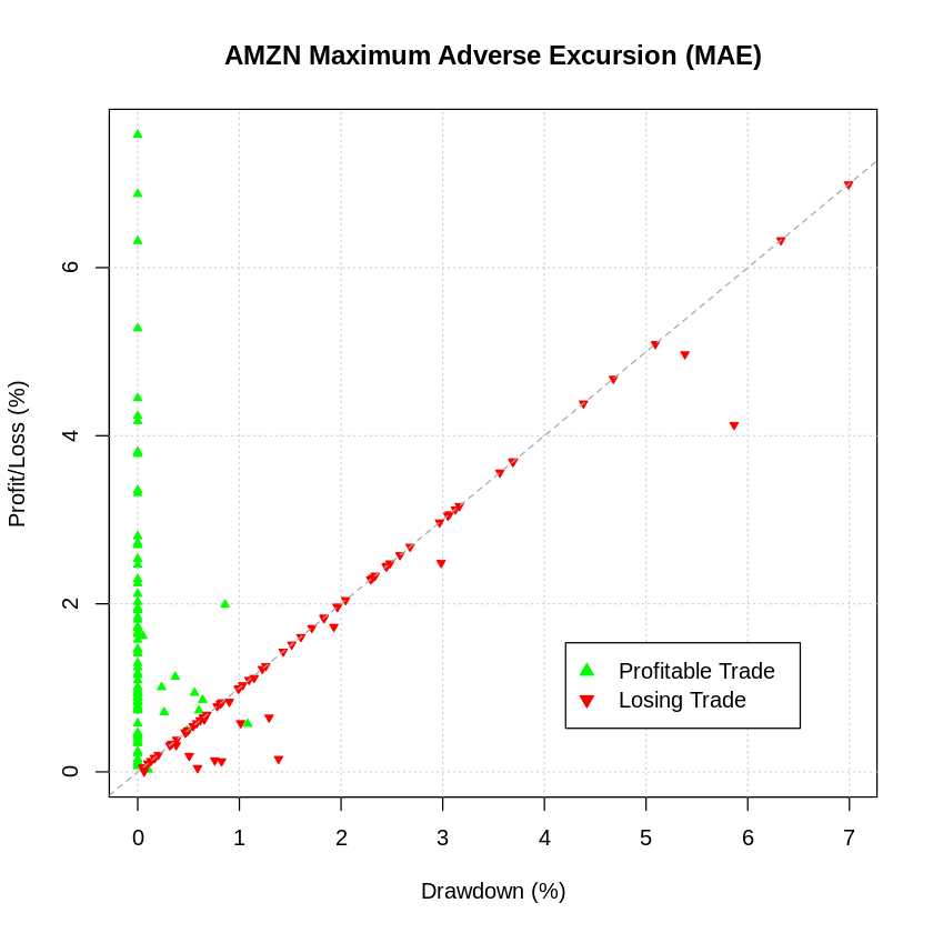
chart.ME(Portfolio = portfolio.st, Symbol = symbol, type = "MAE", scale = "percent")

[24]:

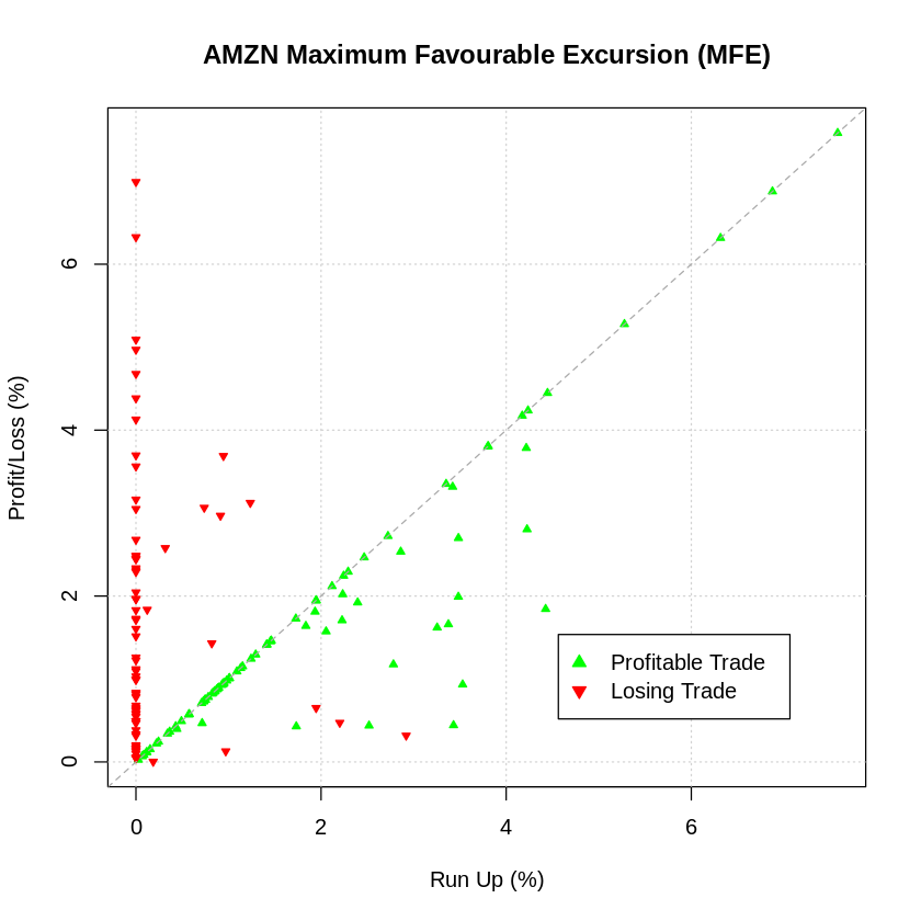
chart.ME(Portfolio = portfolio.st, Symbol = symbol, type = "MFE", scale = "percent")

Moving Average Crossover Strategy - Sample 2

when the short term moving average crosses above the long term moving average, this indicates a buy signal
when the short term moving average crosses below the long term moving average, it may be a good moment to sell

Reference: https://towardsdatascience.com/making-a-trade-call-using-simple-moving-average-sma-crossover-strategy-python-implementation-29963326da7a

[25]:

# Moving Average Crossover Strategy - Sample 2
# strategy resetting
rm.strat("my strategy")
out <- initPortf(portfolio.st, symbols = symbol, initDate = start, currency = "USD")
out <- initAcct(account.st, portfolios = portfolio.st, initDate = start, currency = "USD", initEq = initEquity)
initOrders(portfolio.st, initDate = start)
strategy(strategy.st, store = TRUE)
# Indicators
out <- add.indicator(strategy.st, name = "SMA", arguments = list(x = quote(Cl(AMZN)), n = 20, maType = "SMA"), label = "SMA20periods")
out <- add.indicator(strategy.st, name = "SMA", arguments = list(x = quote(Cl(AMZN)), n = 50, maType = "SMA"), label = "SMA50periods")
out <- add.indicator(strategy.st, name = "EMA", arguments = list(x = quote(Cl(AMZN)), n = 20, maType = "EMA"), label = "EMA20periods")
out <- add.indicator(strategy.st, name = "EMA", arguments = list(x = quote(Cl(AMZN)), n = 50, maType = "EMA"), label = "EMA50periods")
# Signals
#out <- add.signal(strategy.st, name = "sigCrossover", arguments = list(columns = c("SMA20periods", "SMA50periods"), relationship = "gte", cross = TRUE), label = "buy")
#out <- add.signal(strategy.st, name = "sigCrossover", arguments = list(columns = c("SMA20periods", "SMA50periods"), relationship = "lte", cross = TRUE), label = "sell")
out <- add.signal(strategy.st, name = "sigCrossover", arguments = list(columns = c("EMA20periods", "EMA50periods"), relationship = "gte", cross = TRUE), label = "buy2")
out <- add.signal(strategy.st, name = "sigCrossover", arguments = list(columns = c("EMA20periods", "EMA50periods"), relationship = "lte", cross = TRUE), label = "sell2")
# Rules
out <- add.rule(strategy.st, name = 'ruleSignal', arguments = list(sigcol = "buy2", sigval = TRUE, orderqty = 100, ordertype = 'market', orderside = 'long'), type = 'enter')
out <- add.rule(strategy.st, name = 'ruleSignal', arguments = list(sigcol = "sell2", sigval = TRUE, orderqty = 'all', ordertype = 'market', orderside = 'long'), type = 'exit')
#out <- add.rule(strategy.st, name = 'ruleSignal', arguments = list(sigcol = "sell2", sigval = TRUE, orderqty = -100, ordertype = 'market', orderside = 'short'), type = 'enter')
#out <- add.rule(strategy.st, name = 'ruleSignal', arguments = list(sigcol = "buy2", sigval = TRUE, orderqty = 'all', ordertype = 'market', orderside = 'short'), type = 'exit')

[26]:

# backtesting
applyStrategy(strategy.st, portfolios=portfolio.st)
out <- updatePortf(portfolio.st)
dateRange <- time(getPortfolio(portfolio.st)$summary)[-1]
out <- updateAcct(portfolio.st, dateRange)
out <- updateEndEq(account.st)
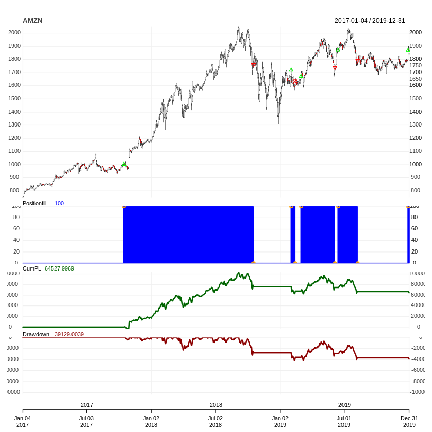
chart.Posn(portfolio.st, Symbol=symbol) #, TA=c("add_SMA(n=20,col='red')"))

[1] "2017-10-16 00:00:00 AMZN 100 @ 1002.940002"
[1] "2018-10-16 00:00:00 AMZN -100 @ 1760.949951"
[1] "2019-02-01 00:00:00 AMZN 100 @ 1718.72998"
[1] "2019-02-13 00:00:00 AMZN -100 @ 1638.01001"
[1] "2019-03-04 00:00:00 AMZN 100 @ 1671.72998"
[1] "2019-06-06 00:00:00 AMZN -100 @ 1738.5"
[1] "2019-06-14 00:00:00 AMZN 100 @ 1870.300049"
[1] "2019-08-08 00:00:00 AMZN -100 @ 1793.400024"
[1] "2019-12-27 00:00:00 AMZN 100 @ 1868.77002"

[27]:

tstats <- tradeStats(portfolio.st, use="trades", inclZeroDays=FALSE)
data.frame(t(tstats))

A data.frame: 32 × 1
	AMZN
	<chr>
Portfolio	my strategy
Symbol	AMZN
Num.Txns	9
Num.Trades	5
Net.Trading.PL	64528
Avg.Trade.PL	12905.6
Med.Trade.PL	-2188
Largest.Winner	75800.99
Largest.Loser	-8071.997
Gross.Profits	82478
Gross.Losses	-17950
Std.Dev.Trade.PL	35660.49
Std.Err.Trade.PL	15947.85
Percent.Positive	40
Percent.Negative	60
Profit.Factor	4.594874
Avg.Win.Trade	41239
Med.Win.Trade	41239
Avg.Losing.Trade	-5983.333
Med.Losing.Trade	-7690.003
Avg.Daily.PL	16679
Med.Daily.PL	-506.5003
Std.Dev.Daily.PL	40007.96
Std.Err.Daily.PL	20003.98
Ann.Sharpe	6.617956
Max.Drawdown	-41021
Profit.To.Max.Draw	1.573048
Avg.WinLoss.Ratio	6.892312
Med.WinLoss.Ratio	5.362677
Max.Equity	103657
Min.Equity	-3664.001
End.Equity	64528

[28]:

#install.packages("magrittr") # package installations are only needed the first time you use it
#install.packages("dplyr")    # alternative installation of the %>%
#library(magrittr) # needs to be run every time you start R and want to use %>%
#library(dplyr)    # alternatively, this also loads %>%
trades <- tstats %>%
    mutate(Trades = Num.Trades,
        Win.Percent = Percent.Positive,
        Loss.Percent = Percent.Negative,
        WL.Ratio = Percent.Positive/Percent.Negative) %>%
    select(Trades, Win.Percent, Loss.Percent, WL.Ratio)
data.frame(t(trades))

A data.frame: 4 × 1
	t.trades.
	<dbl>
Trades	5.0000000
Win.Percent	40.0000000
Loss.Percent	60.0000000
WL.Ratio	0.6666667

[29]:

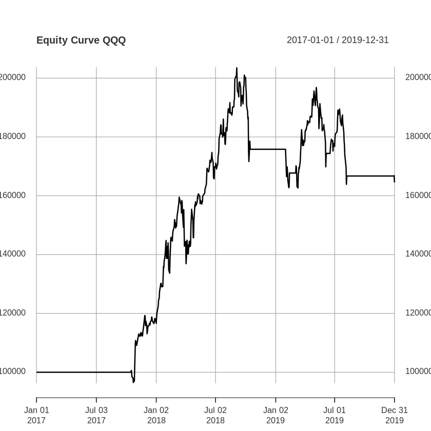
a <- getAccount(account.st)
equity <- a$summary$End.Eq
plot(equity, main = "Equity Curve QQQ")

[30]:

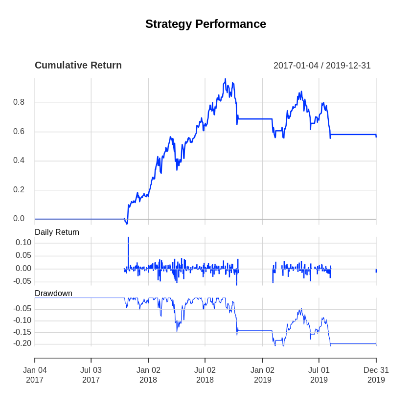
ret <- Return.calculate(equity, method = "log")
charts.PerformanceSummary(ret, colorset = bluefocus, main = "Strategy Performance")

[31]:

rets <- PortfReturns(Account = account.st)
chart.RiskReturnScatter(rets)