Welcome to Backtesting tool comparison’s documentation!
Are you a newbie programmer or you are newbie trader ? This is your tutorial, where you can find some samples of code for downloading of historical data and for backtesting some samples of strategies.
And you may also find some interesting details in the Comparison and Conclusion sections.
Getting started
These contents can help you to start with your quantitative trading (quant trading or QT) system: you can find some samples for the main steps.
There are
many platforms can give you historical data
a lot of program languages that you can use for implementing your strategies
many trading systems that you can use for backtesting your system
Read the documentation on readthedocs for
a sample of the main backtesting steps for a few of the main languages are used for statistical analysis, graphics representation and reporting
comparison among languages and methods for backtesting your strategies
the best practices for your quant trading system
Goals
These contents can be useful at the beginning, when you are newbie programmer.
And it can help you to evaluate which data, language or trading system you need.
Disclaimer
The strategies contained in this tutorial, are some simple samples for having an idea how to use the libraries: those strategies are for the educational purpose only. All investments and trading in the stock market involve risk: any decisions related to buying/selling of stocks or other financial instruments should only be made after a thorough research, backtesting, running in demo and seeking a professional assistance if required.
Contribution
The documentation for R and Python languages, it has been powered by Jupyter:
$ git clone https://github.com/bilardi/backtesting-tool-comparison
$ cd backtesting-tool-comparison/
$ pip install --upgrade -r requirements.txt
$ docker run --rm -p 8888:8888 -e JUPYTER_ENABLE_LAB=yes -v "$PWD":/home/jovyan/ jupyter/datascience-notebook
The images are hosted on S3 and not in this repository:
use a PR for sharing a new version without images, only the new url
it will be our care to move them to S3 with all the others
For testing on your local client the documentation, see this README.md file.
License
These contents are released under the MIT license. See LICENSE for details.
R
Prerequisites
For using the program language R, you have to install r.
For mac,
$ brew install r
There are a lot of guide for getting started with R: knowing the basics will be taken for granted. For installing some packages, you can use RStudio or directly console
$ r
# general tools
install.packages("httr")
install.packages("jsonlite")
install.packages("plotly")
install.packages("devtools")
# for downloading data
install.packages("quantmod") # for Yahoo finance historical data of stock market
install.packages("Quandl")
devtools::install_github("amrrs/coinmarketcapr") # for Crypto currencies
devtools::install_github("amrrs/coindeskr") # for Crypto currencies
# for processing the data: in addition to Quantmod also QuantStrat
devtools::install_github("braverock/blotter")
devtools::install_github("braverock/quantstrat")
If you want to use Jupyter, you can use directly the commands below
$ git clone https://github.com/bilardi/backtesting-tool-comparison
$ cd backtesting-tool-comparison/
$ docker run --rm -p 8888:8888 -e JUPYTER_ENABLE_LAB=yes -v "$PWD":/home/jovyan/ jupyter/r-notebook
Jupyter is very easy for having a GUI virtual environment: knowing the basics will be taken for granted.
You can find all scripts descripted in this tutorial on GitHub:
the .r files in src/r/ folder, the script that you can use on RStudio
the .ipynb files in docs/sources/r/ folder, that you can use on Jupyter or browse on this tutorial
Getting started
R is a programming language and software environment for statistical analysis, graphics representation and reporting.
This is a summary of the r language syntax: you can find more details in cran documentation.
Basics
[1]:
# initialization of a variable
my_numeric_variable <- 1
my_string_variable <- "hello"
# print a variable
my_numeric_variable # and type enter
print(my_string_variable)
[1] "hello"
Vectors
[2]:
# initialization of a vector
my_numeric_vector <- c(1,2,3,4,5,6)
my_sequence <- 1:25
my_string_vector <- c("hello", "world", "!")
my_logic_vector <- c(TRUE, FALSE, T, F)
assign("my_vector", c(1:6))
my_random_vector <- sample(1:5000, 25) # Vector with 25 elements with random number from 1 to 5000
[3]:
# operations with vectors
sum(my_numeric_vector)
mean(my_numeric_vector)
median(my_numeric_vector)
[4]:
# multiplication 2 with each element of a vector
my_vector*2
# division 2 with each element of a vector
my_vector/2
- 2
- 4
- 6
- 8
- 10
- 12
- 0.5
- 1
- 1.5
- 2
- 2.5
- 3
[5]:
# sum each element of a vector with another vector by position
my_new_vector <- my_numeric_vector + my_vector # allow
my_new_vector <- my_numeric_vector + my_sequence # allow but with warning
my_new_vector <- my_numeric_vector + c(1:5) # allow but with warning
Warning message in my_numeric_vector + my_sequence:
“longer object length is not a multiple of shorter object length”
Warning message in my_numeric_vector + c(1:5):
“longer object length is not a multiple of shorter object length”
[6]:
# get element from a vector
my_string_vector[1] # print hello
my_string_vector[-2] # print hello!
my_string_vector[1:2] # print hello world
my_string_vector[c(1,3)] # print hello!
- 'hello'
- '!'
- 'hello'
- 'world'
- 'hello'
- '!'
[7]:
# add labels to a vector
names(my_vector) <- c("one","two","three","four","five","six")
print(my_vector)
one two three four five six
1 2 3 4 5 6
[8]:
# get data type of a vector
class(my_vector) # print integer
typeof(my_string_vector) # print character
mode(my_vector) # print numeric
[9]:
# convertion of each element of a vector
as.character(my_vector)
- '1'
- '2'
- '3'
- '4'
- '5'
- '6'
Matrixes
A matrix is a vector with more dimensions
[10]:
# matrix
my_matrix <- matrix(1:10, nrow = 2, ncol = 5) # creates a matrix bidimensional with 2 rows and 5 columns
my_matrix
my_matrix[2,2] # prints 4
my_matrix[1,] # prints row 1
my_matrix[,2] # prints column 2
| 1 | 3 | 5 | 7 | 9 |
| 2 | 4 | 6 | 8 | 10 |
- 1
- 3
- 5
- 7
- 9
- 3
- 4
[11]:
# merge of vectors
vector_one <- c("one", 0.1)
vector_two <- c("two", 1)
vector_three <- c("three", 10)
my_vectors <- matrix(c(vector_one, vector_two, vector_three), nrow = 3, ncol = 2, byrow = 1)
colnames(my_vectors) <- c("vector number", "quantity")
rownames(my_vectors) <- c("yesterday", "today", "tomorrow")
[12]:
my_vectors
| vector number | quantity | |
|---|---|---|
| yesterday | one | 0.1 |
| today | two | 1 |
| tomorrow | three | 10 |
Weighted average
[13]:
# performance
apple_performance <- 3
netflix_performance <- 7
amazon_performance <- 11
# weight
apple_weight <- .3
netflix_weight <- .4
amazon_weight <- .3
# portfolio performance
weighted_average <- apple_performance * apple_weight + netflix_performance * netflix_weight + amazon_performance * amazon_weight
weighted_average
[14]:
# the same sample but with vectors
performance <- c(3,7,11)
weight <- c(.3,.4,.3)
company <- c('apple','netflix','amazon')
names(performance) <- company
names(weight) <- company
performance_weight <- performance * weight
performance_weight
weighted_average <- sum(performance_weight)
weighted_average
- apple
- 0.9
- netflix
- 2.8
- amazon
- 3.3
Functions
[15]:
# the weighted average but with a function
weighted_average_function <- function(performance, weight) {
return(sum(performance * weight))
}
performance <- c(3,7,11)
weight <- c(.3,.4,.3)
weighted_average <- weighted_average_function(performance, weight)
weighted_average
Historical data
This page contains some samples for downloading historical data of your quant trading system.
Quantmod library
Stock markets from Yahoo finance by Quantmod library (doc)
[1]:
library(quantmod)
symbol <- "AMZN"
getSymbols(symbol) # or getSymbols(symbol, src = "yahoo")
Loading required package: xts
Loading required package: zoo
Attaching package: ‘zoo’
The following objects are masked from ‘package:base’:
as.Date, as.Date.numeric
Loading required package: TTR
Registered S3 method overwritten by 'quantmod':
method from
as.zoo.data.frame zoo
‘getSymbols’ currently uses auto.assign=TRUE by default, but will
use auto.assign=FALSE in 0.5-0. You will still be able to use
‘loadSymbols’ to automatically load data. getOption("getSymbols.env")
and getOption("getSymbols.auto.assign") will still be checked for
alternate defaults.
This message is shown once per session and may be disabled by setting
options("getSymbols.warning4.0"=FALSE). See ?getSymbols for details.
[2]:
head(AMZN) # returns some data of AMZN vector
AMZN.Open AMZN.High AMZN.Low AMZN.Close AMZN.Volume AMZN.Adjusted
2007-01-03 38.68 39.06 38.05 38.70 12405100 38.70
2007-01-04 38.59 39.14 38.26 38.90 6318400 38.90
2007-01-05 38.72 38.79 37.60 38.37 6619700 38.37
2007-01-08 38.22 38.31 37.17 37.50 6783000 37.50
2007-01-09 37.60 38.06 37.34 37.78 5703000 37.78
2007-01-10 37.49 37.70 37.07 37.15 6527500 37.15
[3]:
colnames(AMZN) # returns column names of AMZN vector
- 'AMZN.Open'
- 'AMZN.High'
- 'AMZN.Low'
- 'AMZN.Close'
- 'AMZN.Volume'
- 'AMZN.Adjusted'
[4]:
#Op(AMZN) # only column of open of all data
#Hi(AMZN) # only column of high of all data
#Lo(AMZN) # only column of low of all data
#Cl(AMZN) # only column of close of all data
#Vo(AMZN) # only column of volume of all data
#Ad(AMZN) # value adjusted of the close (of all data)
#OHLC(AMZN) # columns open, high, low and close of all data
Exchange rates (forex) from Yahoo finance
[5]:
library(quantmod)
cross_from <- c("EUR", "USD", "CAD")
cross_to <- c("USD", "JPY", "USD")
getQuote(paste0(cross_from, cross_to, "=X"))
| Trade Time | Last | Change | % Change | Open | High | Low | Volume | |
|---|---|---|---|---|---|---|---|---|
| <dttm> | <dbl> | <dbl> | <dbl> | <dbl> | <dbl> | <dbl> | <int> | |
| EURUSD=X | 2021-01-11 12:21:43 | 1.2162491 | -0.006693244 | -0.5473087 | 1.2226434 | 1.2239902 | 1.2158055 | 0 |
| USDJPY=X | 2021-01-11 12:22:10 | 104.2400000 | 0.291000370 | 0.2799453 | 103.9490000 | 104.2490000 | 103.6870000 | 0 |
| CADUSD=X | 2021-01-11 12:22:10 | 0.7822278 | -0.006048977 | -0.7673632 | 0.7882768 | 0.7886435 | 0.7822095 | 0 |
Exchange rates (forex) from Oanda
[6]:
library(quantmod)
currency <- "EUR/GBP"
# the last 6 months
getSymbols(currency, src = "oanda")
head(EURGBP) # returns some data of EURGBP vector
EUR.GBP
2020-07-16 0.907685
2020-07-17 0.909031
2020-07-18 0.909320
2020-07-19 0.909368
2020-07-20 0.907640
2020-07-21 0.903154
[7]:
# the last 60 days
getSymbols(currency, from = Sys.Date() - 60, to = Sys.Date(), src = "oanda")
head(EURGBP) # returns some data of EURGBP vector
EUR.GBP
2020-11-12 0.895798
2020-11-13 0.898187
2020-11-14 0.896580
2020-11-15 0.896644
2020-11-16 0.897208
2020-11-17 0.896298
CoinMarketCap API
Crypto currencies by coinmarketcap (doc) and coindeskr (doc) Many libraries are not supported for a long period or it may no longer be supported because it has violated a policy:
the library coindeskr has violated the CRAN’s policy and it has archived on 2020-09-04
its GitHub repository is already available, but it has not updated for a change of CoinMarketCap API
[8]:
library(coinmarketcapr)
library(coindeskr)
last_marketcap <- get_global_marketcap("EUR")
today_marketcap <- get_marketcap_ticker_all()
head(today_marketcap[,1:8])
last_month <- get_last31days_price() # default it is Bitcoin
current_price <- get_current_price() # default it is Bitcoin
⚠ The old API is used when no 'apikey' is given.
Error: lexical error: invalid char in json text.
<!DOCTYPE HTML> <html lang="en-
(right here) ------^
Traceback:
1. get_global_marketcap("EUR")
2. check_response(d)
3. stop(cat(crayon::red(cli::symbol$cross, "The request was not succesfull! \n",
. "Request URL:\n", req$url, "\n", "Response Content:\n", jsonlite::prettify(rawToChar(req$content)),
. "\n")))
4. cat(crayon::red(cli::symbol$cross, "The request was not succesfull! \n",
. "Request URL:\n", req$url, "\n", "Response Content:\n", jsonlite::prettify(rawToChar(req$content)),
. "\n"))
5. crayon::red(cli::symbol$cross, "The request was not succesfull! \n",
. "Request URL:\n", req$url, "\n", "Response Content:\n", jsonlite::prettify(rawToChar(req$content)),
. "\n")
6. mypaste(...)
7. lapply(list(...), as.character)
8. jsonlite::prettify(rawToChar(req$content))
9. reformat(txt, TRUE, indent_string = paste(rep(" ", as.integer(indent)),
. collapse = ""))
10. stop(out[[2]], call. = FALSE)
11. base::stop(..., call. = FALSE)
Below you can find a sample with sandbox API of CoinMarketCap.
[9]:
library(httr)
library(jsonlite)
base_url <- 'https://sandbox-api.coinmarketcap.com/'
get_coinmarketcap_data <- function(base_url, path, query) {
response <- GET(url = base_url, path = paste('v1/', path, sep = ''), query = query)
content <- content(response, 'text', encoding = 'utf-8')
return(fromJSON(content, flatten = TRUE))
}
# returns all active cryptocurrencies
path <- 'cryptocurrency/map'
marketcap_map <- get_coinmarketcap_data(base_url, path, list())
head(marketcap_map$data)
| id | name | symbol | slug | is_active | rank | platform.id | platform.name | platform.symbol | platform.slug | platform.token_address | |
|---|---|---|---|---|---|---|---|---|---|---|---|
| <int> | <chr> | <chr> | <chr> | <int> | <int> | <int> | <chr> | <chr> | <chr> | <chr> | |
| 1 | 1 | Bitcoin | BTC | bitcoin | 1 | 1 | NA | NA | NA | NA | NA |
| 2 | 2 | Litecoin | LTC | litecoin | 1 | 5 | NA | NA | NA | NA | NA |
| 3 | 3 | Namecoin | NMC | namecoin | 1 | 310 | NA | NA | NA | NA | NA |
| 4 | 4 | Terracoin | TRC | terracoin | 1 | 926 | NA | NA | NA | NA | NA |
| 5 | 5 | Peercoin | PPC | peercoin | 1 | 346 | NA | NA | NA | NA | NA |
| 6 | 6 | Novacoin | NVC | novacoin | 1 | 842 | NA | NA | NA | NA | NA |
[10]:
# returns last market data of all active cryptocurrencies
path <- 'cryptocurrency/listings/latest'
query <- list(convert = 'EUR')
last_marketcap <- get_coinmarketcap_data(base_url, path, query)
head(last_marketcap$data)
| id | name | symbol | slug | num_market_pairs | date_added | tags | max_supply | circulating_supply | total_supply | ⋯ | platform.symbol | platform.slug | platform.token_address | quote.EUR.price | quote.EUR.volume_24h | quote.EUR.percent_change_1h | quote.EUR.percent_change_24h | quote.EUR.percent_change_7d | quote.EUR.market_cap | quote.EUR.last_updated | |
|---|---|---|---|---|---|---|---|---|---|---|---|---|---|---|---|---|---|---|---|---|---|
| <int> | <chr> | <chr> | <chr> | <int> | <chr> | <list> | <dbl> | <dbl> | <dbl> | ⋯ | <chr> | <chr> | <chr> | <dbl> | <dbl> | <lgl> | <lgl> | <lgl> | <dbl> | <chr> | |
| 1 | 1 | Bitcoin | BTC | bitcoin | 7919 | 2013-04-28T00:00:00.000Z | mineable | 2.1e+07 | 17906012 | 17906012 | ⋯ | NA | NA | NA | 8708.4427303 | 12507935648 | NA | NA | NA | 155933480030 | 2019-08-30T18:51:01.000Z |
| 2 | 1027 | Ethereum | ETH | ethereum | 5629 | 2015-08-07T00:00:00.000Z | mineable | NA | 107537936 | 107537936 | ⋯ | NA | NA | NA | 153.6859725 | 5260772807 | NA | NA | NA | 16527072336 | 2019-08-30T18:51:01.000Z |
| 3 | 52 | XRP | XRP | ripple | 449 | 2013-08-04T00:00:00.000Z | 1.0e+11 | 42932866967 | 99991366793 | ⋯ | NA | NA | NA | 0.2318186 | 844359719 | NA | NA | NA | 9952638454 | 2019-08-30T18:51:01.000Z | |
| 4 | 1831 | Bitcoin Cash | BCH | bitcoin-cash | 378 | 2017-07-23T00:00:00.000Z | mineable | 2.1e+07 | 17975975 | 17975975 | ⋯ | NA | NA | NA | 256.0351264 | 1281819319 | NA | NA | NA | 4602481031 | 2019-08-30T18:51:01.000Z |
| 5 | 2 | Litecoin | LTC | litecoin | 538 | 2013-04-28T00:00:00.000Z | mineable | 8.4e+07 | 63147124 | 63147124 | ⋯ | NA | NA | NA | 58.6260748 | 2207389317 | NA | NA | NA | 3702068016 | 2019-08-30T18:51:01.000Z |
| 6 | 825 | Tether | USDT | tether | 3016 | 2015-02-25T00:00:00.000Z | NA | 4008269411 | 4095057493 | ⋯ | OMNI | omni | 31 | 0.9138714 | 14536357084 | NA | NA | NA | 3663042762 | 2019-08-30T18:51:01.000Z |
[11]:
# returns last market data of Bitcoin
path <- 'cryptocurrency/quotes/latest'
query <- list(id = 1, convert = 'EUR')
last_bitcoin <- get_coinmarketcap_data(base_url, path, query)
last_bitcoin$data$`1`
last_bitcoin$data$`1`$`quote`$EUR
- $id
- 1
- $name
- 'Bitcoin'
- $symbol
- 'BTC'
- $slug
- 'bitcoin'
- $num_market_pairs
- 7919
- $date_added
- '2013-04-28T00:00:00.000Z'
- $tags
- 'mineable'
- $max_supply
- 21000000
- $circulating_supply
- 17906012
- $total_supply
- 17906012
- $is_active
- 1
- $is_market_cap_included_in_calc
- 1
- $platform
- NULL
- $cmc_rank
- 1
- $is_fiat
- 0
- $last_updated
- '2019-08-30T18:51:28.000Z'
- $quote
- $EUR =
- $price
- 8708.44273026964
- $volume_24h
- 12507935648.1974
- $percent_change_1h
- NULL
- $percent_change_24h
- NULL
- $percent_change_7d
- NULL
- $market_cap
- 155933480029.521
- $last_updated
- '2019-08-30T18:51:01.000Z'
- $price
- 8708.44273026964
- $volume_24h
- 12507935648.1974
- $percent_change_1h
- NULL
- $percent_change_24h
- NULL
- $percent_change_7d
- NULL
- $market_cap
- 155933480029.521
- $last_updated
- '2019-08-30T18:51:01.000Z'
[12]:
# returns historical data from a time_start to a time_end
path <- 'cryptocurrency/quotes/historical'
query <- list(id = 1, convert = 'EUR', time_start = '2020-05-21T12:14', time_end = '2020-05-21T12:44')
data <- get_coinmarketcap_data(base_url, path, query)
head(data$data)
- $id
- 1
- $name
- 'Bitcoin'
- $symbol
- 'BTC'
- $is_fiat
- 0
- $quotes
A data.frame: 6 × 2 timestamp quote.EUR.timestamp <chr> <chr> 1 2020-05-21T12:19:03.000Z 2020-05-21T12:19:03.000Z 2 2020-05-21T12:24:02.000Z 2020-05-21T12:24:02.000Z 3 2020-05-21T12:29:03.000Z 2020-05-21T12:29:03.000Z 4 2020-05-21T12:34:03.000Z 2020-05-21T12:34:03.000Z 5 2020-05-21T12:39:01.000Z 2020-05-21T12:39:01.000Z 6 2020-05-21T12:44:02.000Z 2020-05-21T12:44:02.000Z
Quandl library
OHLC (Open High Low Close) data by Quandl library (doc), for example crude oil
[13]:
library(Quandl)
oil_data <- Quandl(code = "CHRIS/CME_QM1")
head(oil_data) # returns all free columns names
| Date | Open | High | Low | Last | Change | Settle | Volume | Previous Day Open Interest | |
|---|---|---|---|---|---|---|---|---|---|
| <date> | <dbl> | <dbl> | <dbl> | <dbl> | <dbl> | <dbl> | <dbl> | <dbl> | |
| 1 | 2021-01-08 | 50.925 | 52.750 | 50.825 | 52.750 | 1.41 | 52.24 | 10770 | 1833 |
| 2 | 2021-01-07 | 50.525 | 51.275 | 50.400 | 50.950 | 0.20 | 50.83 | 10814 | 1800 |
| 3 | 2021-01-06 | 49.825 | 50.925 | 49.475 | 50.525 | 0.70 | 50.63 | 16675 | 1908 |
| 4 | 2021-01-05 | 47.400 | 50.200 | 47.275 | 49.850 | 2.31 | 49.93 | 23473 | 1799 |
| 5 | 2021-01-04 | 48.400 | 49.850 | 47.200 | 47.350 | -0.90 | 47.62 | 21845 | 1350 |
| 6 | 2020-12-31 | 48.325 | 48.575 | 47.775 | 48.450 | 0.12 | 48.52 | 6698 | 1446 |
[14]:
#getPrice(oil_data) # returns all free columns values
#getPrice(oil_data, symbol = "CHRIS/CME_QM1", prefer = "Open$") # returns open values of a specific symbol
getPrice(oil_data, prefer = "Open$") # returns open values
- 50.925
- 50.525
- 49.825
- 47.4
- 48.4
- 48.325
- 48.125
- 47.7
- 48.2
- 48.1
- 46.775
- 47.85
- 49.3
- 48.35
- 47.825
- 47.55
- 47.05
- 46.65
- 47
- 45.725
- 45.55
- 45.6
- 46.125
- 45.625
- 45
- 44.375
- 45.05
- 45.45
- 45.9
- 44.8
- 42.825
- 42.55
- 41.85
- 41.6
- 41.325
- 41.525
- 40.175
- 40.9
- 41.425
- 41.8
- 39.825
- 37.325
- 38.5
- 39.1
- 38.15
- 37.025
- 35.325
- 36.1
- 37.475
- 38.95
- 38.625
- 39.75
- 40.6
- 40.025
- 41.25
- 40.95
- 40.9
- 40.875
- 41.15
- 40.225
- 39.525
- 40.45
- 41.325
- 39.975
- 39.875
- 39.375
- 37
- 38.525
- 39.85
- 39.225
- 40.575
- 40.125
- 40.175
- 39.6
- 39.725
- 39.875
- 40.85
- 40.95
- 40.175
- 38.325
- 37.3
- 37.325
- 37.1
- 37.8
- 36.85
- 39.45
- 41.25
- 41.575
- 43.05
- 42.825
- 42.925
- 43
- 43.475
- 43.375
- 42.375
- 42.425
- 42.75
- 42.95
- 42.65
- 42.65
- 42.15
- 42.325
- 42.55
- 41.575
- 42
- 41.55
- 41.925
- 42.225
- 41.525
- 40.775
- 40.375
- 40.4
- 41.325
- 41.1
- 41.675
- 41.325
- 41.1
- 41.925
- 41.55
- 40.8
- 40.45
- 40.75
- 40.95
- 40.55
- 39.625
- 40.375
- 39.6
- 40.825
- 40.45
- 40.6
- 40.375
- 39.775
- 39.825
- 39.625
- 37.95
- 39.075
- 38.05
- 39.975
- 40.65
- 39.05
- 38.875
- 37.625
- 37.95
- 37.1
- 35.975
- 36.25
- 39.05
- 38.425
- 38.2
- 39.4
- 37.325
- 36.725
- 36.825
- 35.525
- 35.075
- 33.675
- 32.025
- 34.1
- 33.3
- 33.95
- 33.5
- 31.9
- 32.35
- 30
- 27.575
- 25.7
- 25.35
- 24.575
- 24.425
- 23.5
- 24
- 25.5
- 21.15
- 19.1
- 19.075
- 15.6
- 13.275
- 13
- 16.875
- 16.825
- 14.3
- 13
- 21.3
- 17.75
- 20.025
- 20.125
- 20.7
- 22.4
- 24.55
- 26.25
- 24.25
- 26.35
- 26.5
- 24.8
- 21.225
- 20.1
- 20.25
- 21
- 23.3
- 24.15
- ⋯
- 56.1
- 55.375
- 55.325
- 57.25
- 59.225
- 63.35
- 63
- 65.525
- 66.725
- 67.4
- 67.6
- 69.25
- 66.125
- 73.5
- 73.85
- 75.5
- 76.575
- 76.325
- 74.325
- 74.225
- 75.525
- 75.95
- 74.3
- 76.9
- 77.5
- 77.275
- 78.475
- 77.9
- 78.9
- 77.4
- 78.175
- 80.6
- 81
- 81.925
- 81.575
- 80.65
- 81.225
- 81.925
- 80.4
- 82.525
- 81.85
- 82.4
- 83.175
- 80.95
- 82.3
- 85.025
- 85.3
- 84.4
- 87.7
- 88.45
- 90.5
- 89.75
- 91.35
- 90.725
- 91.375
- 94.3
- 93.3
- 92.525
- 92.9
- 91.65
- 90.7
- 91.625
- 91.95
- 94
- 94.725
- 92.75
- 92.125
- 93.05
- 91.7
- 92.775
- 93.15
- 93.45
- 94.525
- 95.1
- 93.225
- 95.875
- 94.575
- 93.725
- 93.875
- 93.35
- 93.375
- 93.9
- 93.475
- 92.85
- 93.925
- 97.2
- 95.525
- 97.35
- 97.175
- 97.85
- 97.45
- 97.6
- 96.9
- 97.6
- 98.4
- 97.675
- 97.65
- 99.525
- 101
- 101.575
- 101.875
- 102.05
- 103.2
- 102
- 102.75
- 101.725
- 103.75
- 101.475
- 100.2
- 100.95
- 100.525
- 102.85
- 101.95
- 103.5
- 103.4
- 103.8
- 104.275
- 105.225
- 105.55
- 105.775
- 105.65
- 106.7
- 106.025
- 106
- 106.9
- 106.075
- 105.7
- 106.625
- 106.575
- 106.9
- 106.825
- 104.5
- 104.325
- 104.5
- 102.7
- 102.425
- 102.375
- 102.775
- 102.45
- 102.875
- 103.45
- 103.075
- 104.15
- 104.375
- 103.75
- 103.825
- 102.925
- 102.1
- 101.6
- 101.575
- 102
- 101.925
- 100.6
- 100.025
- 100.25
- 100.775
- 99.825
- 99.425
- 99.95
- 99.2
- 99.7
- 100.775
- 100.85
- 100.25
- 101.925
- 101.5
- 101.9
- 103.625
- 103.65
- 103.825
- 103.825
- 103.6
- 103.65
- 103.35
- 103.4
- 102.325
- 100.7
- 101
- 100.4
- 99.3
- 99.675
- 101.5
- 101.575
- 101.325
- 100.275
- 99.2
- 99.425
- 99.45
- 98.675
- 99.15
- 98.575
- 98.025
- 99.35
- 98.2
- 98.1
- 99.5
- 100.925
- 101.9
- 101
- 103.325
Graphics
This is a sample for plotting with R.
[1]:
library(quantmod)
# initialization
symbols = c("AMZN", "FB", "NFLX", "MSFT")
start <- as.Date("2017-01-01")
end <- as.Date("2020-01-01")
getSymbols(Symbols = symbols, src = "yahoo", from = start, to = end)
# get only Close values of AMZN and MSFT symbols
stocks <- as.xts(data.frame(AMZN = AMZN[,"AMZN.Close"], MSFT = MSFT[,"MSFT.Close"]))
Loading required package: xts
Loading required package: zoo
Attaching package: ‘zoo’
The following objects are masked from ‘package:base’:
as.Date, as.Date.numeric
Loading required package: TTR
Registered S3 method overwritten by 'quantmod':
method from
as.zoo.data.frame zoo
‘getSymbols’ currently uses auto.assign=TRUE by default, but will
use auto.assign=FALSE in 0.5-0. You will still be able to use
‘loadSymbols’ to automatically load data. getOption("getSymbols.env")
and getOption("getSymbols.auto.assign") will still be checked for
alternate defaults.
This message is shown once per session and may be disabled by setting
options("getSymbols.warning4.0"=FALSE). See ?getSymbols for details.
- 'AMZN'
- 'FB'
- 'NFLX'
- 'MSFT'
[2]:
# plotting
library(plotly)
plot(AMZN[,"AMZN.Close"], main = "AMZN") # prints linear graph
Loading required package: ggplot2
Attaching package: ‘plotly’
The following object is masked from ‘package:ggplot2’:
last_plot
The following object is masked from ‘package:stats’:
filter
The following object is masked from ‘package:graphics’:
layout

[3]:
# create a custom theme
my_theme <- chart_theme()
my_theme$col$up.col <- "darkgreen"
my_theme$col$up.border <- "black"
my_theme$col$dn.col <- "darkred"
my_theme$col$dn.border <- "black"
my_theme$rylab <- FALSE
my_theme$col$grid <- "lightgrey"
[4]:
# using the custom theme with a range
chart_Series(AMZN, subset = "2017-10::2018-09", theme = my_theme)

[5]:
# using the custom theme with a range of one month
chart_Series(AMZN, subset = "2018-09", theme = my_theme)

[6]:
# using the black theme of quantmod
barChart(AMZN, theme = chartTheme('black'))

[7]:
# using the candle theme of quantmod
candleChart(AMZN, up.col = "green", dn.col = "red", theme = "white")

[8]:
# zoom of graph on one month
zoomChart("2018-09")

[9]:
# zoom of graph on one year
zoomChart("2018")

[10]:
# add indicators
addSMA(n = c(20, 50, 200)) # adds simple moving averages

[11]:
addBBands(n = 20, sd = 2, ma = "SMA", draw = "bands", on = -1) # sd = standard deviation, ma = average

[12]:
AMZN_ema_21 <- EMA(Cl(AMZN), n=21) # exponencial moving average
addTA(AMZN_ema_21, on = 1, col = "red")

[13]:
AMZN_ema_50 <- EMA(Cl(AMZN), n=50) # exponencial moving average
addTA(AMZN_ema_50, on = 1, col = "blue")

[14]:
AMZN_ema_200 <- EMA(Cl(AMZN), n=200) # exponencial moving average
addTA(AMZN_ema_200, on = 1, col = "orange")

[15]:
addRSI(n = 14, maType = "EMA", wilder = TRUE) # relative strength index

Strategies
You can initilize a strategy by R language.
The main libraries are
QuantStrat, for managing the strategy
PerformanceAnalytics, for performance and risk analysis
How to load indicators on your strategy
[1]:
#install.packages("quantmod")
#require(devtools)
#devtools::install_github("braverock/blotter")
#devtools::install_github("braverock/quantstrat")
[2]:
library(quantmod)
# initialization
Sys.setenv(TZ="UTC")
symbol = as.character("AMZN")
start <- as.Date("2017-01-01")
end <- as.Date("2020-01-01")
getSymbols(Symbols = symbol, src = "yahoo", from = start, to = end)
Loading required package: xts
Loading required package: zoo
Attaching package: ‘zoo’
The following objects are masked from ‘package:base’:
as.Date, as.Date.numeric
Loading required package: TTR
Registered S3 method overwritten by 'quantmod':
method from
as.zoo.data.frame zoo
‘getSymbols’ currently uses auto.assign=TRUE by default, but will
use auto.assign=FALSE in 0.5-0. You will still be able to use
‘loadSymbols’ to automatically load data. getOption("getSymbols.env")
and getOption("getSymbols.auto.assign") will still be checked for
alternate defaults.
This message is shown once per session and may be disabled by setting
options("getSymbols.warning4.0"=FALSE). See ?getSymbols for details.
[3]:
AMZN <- na.omit(lag(AMZN))
# calculate indicators
sma20 <- SMA(Cl(AMZN), n = 20)
ema20 <- EMA(Cl(AMZN), n = 20)
[4]:
library(quantstrat)
# strategy initialization
currency("USD")
stock(symbol, currency = 'USD', multiplier = 1)
tradeSize <- 100000
initEquity <- 100000
account.st <- portfolio.st <- strategy.st <- "my strategy"
rm.strat("my strategy")
out <- initPortf(portfolio.st, symbols = symbol, initDate = start, currency = "USD")
out <- initAcct(account.st, portfolios = portfolio.st, initDate = start, currency = "USD", initEq = initEquity)
initOrders(portfolio.st, initDate = start)
strategy(strategy.st, store = TRUE)
Loading required package: blotter
Loading required package: FinancialInstrument
Loading required package: PerformanceAnalytics
Attaching package: ‘PerformanceAnalytics’
The following object is masked from ‘package:graphics’:
legend
Loading required package: foreach
[5]:
# indicators with QuantStrat
out <- add.indicator(strategy.st, name = "SMA", arguments = list(x = quote(Cl(AMZN)), n = 20, maType = "SMA"), label = "SMA20periods")
out <- add.indicator(strategy.st, name = "SMA", arguments = list(x = quote(Cl(AMZN)), n = 50, maType = "SMA"), label = "SMA50periods")
out <- add.indicator(strategy.st, name = "EMA", arguments = list(x = quote(Cl(AMZN)), n = 20, maType = "EMA"), label = "EMA20periods")
out <- add.indicator(strategy.st, name = "EMA", arguments = list(x = quote(Cl(AMZN)), n = 50, maType = "EMA"), label = "EMA50periods")
out <- add.indicator(strategy.st, name = "RSI", arguments = list(price = quote(Cl(AMZN)), n = 7), label = "RSI720periods")
out <- add.indicator(strategy.st, name = "BBands", arguments = list(HLC = quote(Cl(AMZN)), n = 20, maType = "SMA", sd = 2), label = "Bollinger Bands")
[6]:
# custom indicator
RSIaverage <- function(price, n1, n2) {
RSI_1 <- RSI(price = price, n = n1)
RSI_2 <- RSI(price = price, n = n2)
calculatedAverage <- (RSI_1 + RSI_2) / 2
colnames(calculatedAverage) <- "RSI_average"
return(calculatedAverage)
}
out <- add.indicator(strategy.st, name = "RSIaverage", arguments = list(price = quote(Cl(AMZN)), n1 = 7, n2 = 14), label = "RSIaverage")
[7]:
# first tests
plot(RSIaverage(Cl(AMZN), n1=7, n2=14)) # for graphing your function results

[8]:
# load all indicators on my data
test <- applyIndicators(strategy = strategy.st, mktdata = OHLC(AMZN))
subsetTest <- test["2018-01-01/2019-01-01"]
head(subsetTest)
AMZN.Open AMZN.High AMZN.Low AMZN.Close SMA.SMA20periods
2018-01-02 1182.35 1184.00 1167.50 1169.47 1168.841
2018-01-03 1172.00 1190.00 1170.51 1189.01 1170.174
2018-01-04 1188.30 1205.49 1188.30 1204.20 1173.687
2018-01-05 1205.00 1215.87 1204.66 1209.59 1177.088
2018-01-08 1217.51 1229.14 1210.00 1229.14 1180.927
2018-01-09 1236.00 1253.08 1232.03 1246.87 1185.281
SMA.SMA50periods EMA.EMA20periods EMA.EMA50periods rsi.RSI720periods
2018-01-02 1129.739 1168.779 1130.025 44.92805
2018-01-03 1133.787 1170.706 1132.338 60.65982
2018-01-04 1138.213 1173.896 1135.156 68.75469
2018-01-05 1143.078 1177.295 1138.075 71.20734
2018-01-08 1148.143 1182.233 1141.646 78.38659
2018-01-09 1153.622 1188.389 1145.773 82.89832
dn.Bollinger.Bands mavg.Bollinger.Bands up.Bollinger.Bands
2018-01-02 1140.397 1168.841 1197.286
2018-01-03 1140.596 1170.174 1199.753
2018-01-04 1145.498 1173.687 1201.876
2018-01-05 1148.806 1177.088 1205.370
2018-01-08 1146.863 1180.927 1214.992
2018-01-09 1142.097 1185.281 1228.466
pctB.Bollinger.Bands RSI_average.RSIaverage
2018-01-02 0.5110476 49.34830
2018-01-03 0.8183989 60.54486
2018-01-04 1.0412143 66.72199
2018-01-05 1.0746036 68.64585
2018-01-08 1.2076629 74.50261
2018-01-09 1.2130873 78.45513
How to load signals on your strategy
The best practice is to prepare one column for each signal that you want to use on your strategy. The strategy below use the moving averages that they are SMA and EMA. You can use one or the other.
Disclaimer
The strategies below are some simple samples for having an idea how to use the libraries: those strategies are for the educational purpose only. All investments and trading in the stock market involve risk: any decisions related to buying/selling of stocks or other financial instruments should only be made after a thorough research, backtesting, running in demo and seeking a professional assistance if required.
Moving Average Crossover Strategy - Sample 1
when the price value crosses the MA value from below, it will close any existing short position and go long (buy) one unit of the asset
when the price value crosses the MA value from above, it will close any existing long position and go short (sell) one unit of the asset
Reference: https://www.learndatasci.com/tutorials/python-finance-part-3-moving-average-trading-strategy/
[9]:
# Moving Average Crossover Strategy - Sample 1
signalPosition <- function(price, ma) {
# Taking the difference between the prices and the MA timeseries
price_ma_diff <- price - ma
price_ma_diff[is.na(price_ma_diff)] <- 0 # replace missing signals with no position
# Taking the sign of the difference to determine whether the price or the MA is greater
position <- diff(price_ma_diff)
position[is.na(position)] <- 0 # replace missing signals with no position
colnames(position) <- "Signal_position"
return(position)
}
[10]:
#out <- add.indicator(strategy.st, name = "signalPosition", arguments = list(price = Cl(AMZN), ma = sma20), label = "signalPosition")
out <- add.indicator(strategy.st, name = "signalPosition", arguments = list(price = Cl(AMZN), ma = ema20), label = "signalPosition1")
out <- add.signal(strategy.st, name = "sigThreshold", arguments = list(column = "Signal_position", threshold = 2, relationship = "gte", cross = TRUE), label = "buy1")
out <- add.signal(strategy.st, name = "sigThreshold", arguments = list(column = "Signal_position", threshold = -2, relationship = "lte", cross = TRUE), label = "sell1")
#add.signal(strategy.st, name = "sigThreshold", arguments = list(data = position, column = "AMZN.Close", threshold = 2, relationship = "gte", cross = TRUE), label = "buy1")
#add.signal(strategy.st, name = "sigThreshold", arguments = list(data = position, column = "AMZN.Close", threshold = -2, relationship = "lte", cross = TRUE), label = "sell1")
# Creating rules
out <- add.rule(strategy.st, name = 'ruleSignal', arguments = list(sigcol = "buy1", sigval = TRUE, orderqty = 100, ordertype = 'market', orderside = 'long'), type = 'enter')
out <- add.rule(strategy.st, name = 'ruleSignal', arguments = list(sigcol = "sell1", sigval = TRUE, orderqty = 'all', ordertype = 'market', orderside = 'long'), type = 'exit')
#out <- add.rule(strategy.st, name = 'ruleSignal', arguments = list(sigcol = "sell1", sigval = TRUE, orderqty = -100, ordertype = 'market', orderside = 'short'), type = 'enter')
#out <- add.rule(strategy.st, name = 'ruleSignal', arguments = list(sigcol = "buy1", sigval = TRUE, orderqty = 'all', ordertype = 'market', orderside = 'short'), type = 'exit')
[11]:
# backtesting
applyStrategy(strategy.st, portfolios=portfolio.st)
out <- updatePortf(portfolio.st)
dateRange <- time(getPortfolio(portfolio.st)$summary)[-1]
out <- updateAcct(portfolio.st, dateRange)
out <- updateEndEq(account.st)
chart.Posn(portfolio.st, Symbol=symbol, TA=c("add_SMA(n=20,col='red')"))
[1] "2017-02-02 00:00:00 AMZN 100 @ 832.349976"
[1] "2017-02-07 00:00:00 AMZN -100 @ 807.640015"
[1] "2017-02-09 00:00:00 AMZN 100 @ 819.710022"
[1] "2017-02-14 00:00:00 AMZN 100 @ 836.530029"
[1] "2017-02-17 00:00:00 AMZN 100 @ 844.140015"
[1] "2017-02-23 00:00:00 AMZN 100 @ 855.609985"
[1] "2017-02-24 00:00:00 AMZN -400 @ 852.190002"
[1] "2017-03-01 00:00:00 AMZN 100 @ 845.039978"
[1] "2017-03-02 00:00:00 AMZN -100 @ 853.080017"
[1] "2017-03-03 00:00:00 AMZN 100 @ 848.909973"
[1] "2017-03-06 00:00:00 AMZN -100 @ 849.880005"
[1] "2017-03-10 00:00:00 AMZN 100 @ 853"
[1] "2017-03-16 00:00:00 AMZN -100 @ 852.969971"
[1] "2017-03-22 00:00:00 AMZN 100 @ 843.200012"
[1] "2017-03-23 00:00:00 AMZN -100 @ 848.059998"
[1] "2017-03-24 00:00:00 AMZN 100 @ 847.380005"
[1] "2017-03-30 00:00:00 AMZN 100 @ 874.320007"
[1] "2017-04-04 00:00:00 AMZN 100 @ 891.51001"
[1] "2017-04-06 00:00:00 AMZN 100 @ 909.280029"
[1] "2017-04-10 00:00:00 AMZN -400 @ 894.880005"
[1] "2017-04-12 00:00:00 AMZN 100 @ 902.359985"
[1] "2017-04-13 00:00:00 AMZN -100 @ 896.22998"
[1] "2017-04-19 00:00:00 AMZN 100 @ 903.780029"
[1] "2017-04-21 00:00:00 AMZN -100 @ 902.059998"
[1] "2017-04-26 00:00:00 AMZN 100 @ 907.619995"
[1] "2017-05-01 00:00:00 AMZN 100 @ 924.98999"
[1] "2017-05-04 00:00:00 AMZN -200 @ 941.030029"
[1] "2017-05-10 00:00:00 AMZN 100 @ 952.820007"
[1] "2017-05-12 00:00:00 AMZN -100 @ 947.619995"
[1] "2017-05-16 00:00:00 AMZN 100 @ 957.969971"
[1] "2017-05-17 00:00:00 AMZN -100 @ 966.070007"
[1] "2017-05-18 00:00:00 AMZN 100 @ 944.76001"
[1] "2017-05-19 00:00:00 AMZN -100 @ 958.48999"
[1] "2017-05-22 00:00:00 AMZN 100 @ 959.840027"
[1] "2017-05-24 00:00:00 AMZN 100 @ 971.539978"
[1] "2017-05-26 00:00:00 AMZN 100 @ 993.380005"
[1] "2017-06-01 00:00:00 AMZN -300 @ 994.619995"
[1] "2017-06-06 00:00:00 AMZN 100 @ 1011.340027"
[1] "2017-06-08 00:00:00 AMZN -100 @ 1010.070007"
[1] "2017-06-09 00:00:00 AMZN 100 @ 1010.27002"
[1] "2017-06-12 00:00:00 AMZN -100 @ 978.309998"
[1] "2017-06-15 00:00:00 AMZN 100 @ 976.469971"
[1] "2017-06-16 00:00:00 AMZN -100 @ 964.169983"
[1] "2017-06-20 00:00:00 AMZN 100 @ 995.169983"
[1] "2017-06-22 00:00:00 AMZN -100 @ 1002.22998"
[1] "2017-06-23 00:00:00 AMZN 100 @ 1001.299988"
[1] "2017-06-26 00:00:00 AMZN -100 @ 1003.73999"
[1] "2017-06-30 00:00:00 AMZN 100 @ 975.929993"
[1] "2017-07-03 00:00:00 AMZN -100 @ 968"
[1] "2017-07-07 00:00:00 AMZN 100 @ 965.140015"
[1] "2017-07-10 00:00:00 AMZN -100 @ 978.76001"
[1] "2017-07-11 00:00:00 AMZN 100 @ 996.469971"
[1] "2017-07-13 00:00:00 AMZN -100 @ 1006.51001"
[1] "2017-07-14 00:00:00 AMZN 100 @ 1000.630005"
[1] "2017-07-17 00:00:00 AMZN -100 @ 1001.809998"
[1] "2017-07-19 00:00:00 AMZN 100 @ 1024.449951"
[1] "2017-07-25 00:00:00 AMZN -100 @ 1038.949951"
[1] "2017-07-26 00:00:00 AMZN 100 @ 1039.869995"
[1] "2017-07-27 00:00:00 AMZN -100 @ 1052.800049"
[1] "2017-07-28 00:00:00 AMZN 100 @ 1046"
[1] "2017-07-31 00:00:00 AMZN -100 @ 1020.039978"
[1] "2017-08-03 00:00:00 AMZN 100 @ 995.890015"
[1] "2017-08-07 00:00:00 AMZN -100 @ 987.580017"
[1] "2017-08-08 00:00:00 AMZN 100 @ 992.27002"
[1] "2017-08-11 00:00:00 AMZN -100 @ 956.919983"
[1] "2017-08-15 00:00:00 AMZN 100 @ 983.299988"
[1] "2017-08-18 00:00:00 AMZN -100 @ 960.570007"
[1] "2017-08-24 00:00:00 AMZN 100 @ 958"
[1] "2017-08-25 00:00:00 AMZN -100 @ 952.450012"
[1] "2017-08-30 00:00:00 AMZN 100 @ 954.059998"
[1] "2017-09-06 00:00:00 AMZN -100 @ 965.27002"
[1] "2017-09-08 00:00:00 AMZN 100 @ 979.469971"
[1] "2017-09-12 00:00:00 AMZN -100 @ 977.960022"
[1] "2017-09-13 00:00:00 AMZN 100 @ 982.580017"
[1] "2017-09-18 00:00:00 AMZN -100 @ 986.789978"
[1] "2017-09-22 00:00:00 AMZN 100 @ 964.650024"
[1] "2017-09-25 00:00:00 AMZN -100 @ 955.099976"
[1] "2017-09-29 00:00:00 AMZN 100 @ 956.400024"
[1] "2017-10-06 00:00:00 AMZN 100 @ 980.849976"
[1] "2017-10-12 00:00:00 AMZN -200 @ 995"
[1] "2017-10-13 00:00:00 AMZN 100 @ 1000.929993"
[1] "2017-10-20 00:00:00 AMZN -100 @ 986.609985"
[1] "2017-10-26 00:00:00 AMZN 100 @ 972.909973"
[1] "2017-10-27 00:00:00 AMZN -100 @ 972.429993"
[1] "2017-10-31 00:00:00 AMZN 100 @ 1110.849976"
[1] "2017-11-02 00:00:00 AMZN -100 @ 1103.680054"
[1] "2017-11-07 00:00:00 AMZN 100 @ 1120.660034"
[1] "2017-11-09 00:00:00 AMZN -100 @ 1132.880005"
[1] "2017-11-10 00:00:00 AMZN 100 @ 1129.130005"
[1] "2017-11-13 00:00:00 AMZN -100 @ 1125.349976"
[1] "2017-11-16 00:00:00 AMZN 100 @ 1126.689941"
[1] "2017-11-17 00:00:00 AMZN -100 @ 1137.290039"
[1] "2017-11-20 00:00:00 AMZN 100 @ 1129.880005"
[1] "2017-11-21 00:00:00 AMZN -100 @ 1126.310059"
[1] "2017-11-24 00:00:00 AMZN 100 @ 1156.160034"
[1] "2017-11-30 00:00:00 AMZN -100 @ 1161.27002"
[1] "2017-12-04 00:00:00 AMZN 100 @ 1162.349976"
[1] "2017-12-05 00:00:00 AMZN -100 @ 1133.949951"
[1] "2017-12-07 00:00:00 AMZN 100 @ 1152.349976"
[1] "2017-12-13 00:00:00 AMZN 100 @ 1165.079956"
[1] "2017-12-14 00:00:00 AMZN -200 @ 1164.130005"
[1] "2017-12-18 00:00:00 AMZN 100 @ 1179.140015"
[1] "2017-12-21 00:00:00 AMZN -100 @ 1177.619995"
[1] "2017-12-28 00:00:00 AMZN 100 @ 1182.26001"
[1] "2018-01-03 00:00:00 AMZN -100 @ 1189.01001"
[1] "2018-01-04 00:00:00 AMZN 100 @ 1204.199951"
[1] "2018-01-09 00:00:00 AMZN 100 @ 1246.869995"
[1] "2018-01-12 00:00:00 AMZN -200 @ 1276.680054"
[1] "2018-01-16 00:00:00 AMZN 100 @ 1305.199951"
[1] "2018-01-18 00:00:00 AMZN -100 @ 1295"
[1] "2018-01-24 00:00:00 AMZN 100 @ 1362.540039"
[1] "2018-01-26 00:00:00 AMZN -100 @ 1377.949951"
[1] "2018-01-29 00:00:00 AMZN 100 @ 1402.050049"
[1] "2018-02-05 00:00:00 AMZN -100 @ 1429.949951"
[1] "2018-02-06 00:00:00 AMZN 100 @ 1390"
[1] "2018-02-07 00:00:00 AMZN -100 @ 1442.839966"
[1] "2018-02-08 00:00:00 AMZN 100 @ 1416.780029"
[1] "2018-02-09 00:00:00 AMZN -100 @ 1350.5"
[1] "2018-02-14 00:00:00 AMZN 100 @ 1414.51001"
[1] "2018-02-21 00:00:00 AMZN -100 @ 1468.349976"
[1] "2018-02-22 00:00:00 AMZN 100 @ 1482.920044"
[1] "2018-02-26 00:00:00 AMZN -100 @ 1500"
[1] "2018-02-27 00:00:00 AMZN 100 @ 1521.949951"
[1] "2018-03-01 00:00:00 AMZN -100 @ 1512.449951"
[1] "2018-03-06 00:00:00 AMZN 100 @ 1523.609985"
[1] "2018-03-13 00:00:00 AMZN 100 @ 1598.390015"
[1] "2018-03-15 00:00:00 AMZN -200 @ 1591"
[1] "2018-03-22 00:00:00 AMZN 100 @ 1581.859985"
[1] "2018-03-23 00:00:00 AMZN -100 @ 1544.920044"
[1] "2018-03-28 00:00:00 AMZN 100 @ 1497.050049"
[1] "2018-03-29 00:00:00 AMZN -100 @ 1431.420044"
[1] "2018-04-03 00:00:00 AMZN 100 @ 1371.98999"
[1] "2018-04-04 00:00:00 AMZN -100 @ 1392.050049"
[1] "2018-04-05 00:00:00 AMZN 100 @ 1410.569946"
[1] "2018-04-10 00:00:00 AMZN -100 @ 1406.079956"
[1] "2018-04-11 00:00:00 AMZN 100 @ 1436.219971"
[1] "2018-04-13 00:00:00 AMZN -100 @ 1448.5"
[1] "2018-04-16 00:00:00 AMZN 100 @ 1430.790039"
[1] "2018-04-17 00:00:00 AMZN -100 @ 1441.5"
[1] "2018-04-18 00:00:00 AMZN 100 @ 1503.829956"
[1] "2018-04-24 00:00:00 AMZN -100 @ 1517.859985"
[1] "2018-04-27 00:00:00 AMZN 100 @ 1517.959961"
[1] "2018-05-02 00:00:00 AMZN -100 @ 1582.26001"
[1] "2018-05-03 00:00:00 AMZN 100 @ 1569.680054"
[1] "2018-05-04 00:00:00 AMZN -100 @ 1572.079956"
[1] "2018-05-08 00:00:00 AMZN 100 @ 1600.140015"
[1] "2018-05-10 00:00:00 AMZN -100 @ 1608"
[1] "2018-05-11 00:00:00 AMZN 100 @ 1609.079956"
[1] "2018-05-14 00:00:00 AMZN -100 @ 1602.910034"
[1] "2018-05-18 00:00:00 AMZN 100 @ 1581.76001"
[1] "2018-05-21 00:00:00 AMZN -100 @ 1574.369995"
[1] "2018-05-23 00:00:00 AMZN 100 @ 1581.400024"
[1] "2018-05-24 00:00:00 AMZN -100 @ 1601.859985"
[1] "2018-05-25 00:00:00 AMZN 100 @ 1603.069946"
[1] "2018-05-30 00:00:00 AMZN 100 @ 1612.869995"
[1] "2018-06-01 00:00:00 AMZN 100 @ 1629.619995"
[1] "2018-06-05 00:00:00 AMZN 100 @ 1665.27002"
[1] "2018-06-08 00:00:00 AMZN -400 @ 1689.300049"
[1] "2018-06-14 00:00:00 AMZN 100 @ 1704.859985"
[1] "2018-06-18 00:00:00 AMZN 100 @ 1715.969971"
[1] "2018-06-19 00:00:00 AMZN -200 @ 1723.790039"
[1] "2018-06-21 00:00:00 AMZN 100 @ 1750.079956"
[1] "2018-06-25 00:00:00 AMZN -100 @ 1715.670044"
[1] "2018-06-28 00:00:00 AMZN 100 @ 1660.51001"
[1] "2018-06-29 00:00:00 AMZN -100 @ 1701.449951"
[1] "2018-07-02 00:00:00 AMZN 100 @ 1699.800049"
[1] "2018-07-03 00:00:00 AMZN -100 @ 1713.780029"
[1] "2018-07-05 00:00:00 AMZN 100 @ 1693.959961"
[1] "2018-07-06 00:00:00 AMZN -100 @ 1699.72998"
[1] "2018-07-09 00:00:00 AMZN 100 @ 1710.630005"
[1] "2018-07-13 00:00:00 AMZN 100 @ 1796.619995"
[1] "2018-07-19 00:00:00 AMZN 100 @ 1842.920044"
[1] "2018-07-20 00:00:00 AMZN -300 @ 1812.969971"
[1] "2018-07-26 00:00:00 AMZN 100 @ 1863.609985"
[1] "2018-07-30 00:00:00 AMZN -100 @ 1817.27002"
[1] "2018-07-31 00:00:00 AMZN 100 @ 1779.219971"
[1] "2018-08-01 00:00:00 AMZN -100 @ 1777.439941"
[1] "2018-08-03 00:00:00 AMZN 100 @ 1834.329956"
[1] "2018-08-07 00:00:00 AMZN -100 @ 1847.75"
[1] "2018-08-08 00:00:00 AMZN 100 @ 1862.47998"
[1] "2018-08-14 00:00:00 AMZN -100 @ 1896.199951"
[1] "2018-08-15 00:00:00 AMZN 100 @ 1919.650024"
[1] "2018-08-17 00:00:00 AMZN -100 @ 1886.52002"
[1] "2018-08-23 00:00:00 AMZN 100 @ 1904.900024"
[1] "2018-08-27 00:00:00 AMZN -100 @ 1905.390015"
[1] "2018-08-29 00:00:00 AMZN 100 @ 1932.819946"
[1] "2018-08-31 00:00:00 AMZN 100 @ 2002.380005"
[1] "2018-09-04 00:00:00 AMZN -200 @ 2012.709961"
[1] "2018-09-06 00:00:00 AMZN 100 @ 1994.819946"
[1] "2018-09-07 00:00:00 AMZN -100 @ 1958.310059"
[1] "2018-09-13 00:00:00 AMZN 100 @ 1990"
[1] "2018-09-17 00:00:00 AMZN -100 @ 1970.189941"
[1] "2018-09-20 00:00:00 AMZN 100 @ 1926.420044"
[1] "2018-09-21 00:00:00 AMZN -100 @ 1944.300049"
[1] "2018-09-24 00:00:00 AMZN 100 @ 1915.01001"
[1] "2018-09-25 00:00:00 AMZN -100 @ 1934.359985"
[1] "2018-09-26 00:00:00 AMZN 100 @ 1974.550049"
[1] "2018-09-28 00:00:00 AMZN -100 @ 2012.97998"
[1] "2018-10-01 00:00:00 AMZN 100 @ 2003"
[1] "2018-10-02 00:00:00 AMZN -100 @ 2004.359985"
[1] "2018-10-11 00:00:00 AMZN 100 @ 1755.25"
[1] "2018-10-12 00:00:00 AMZN -100 @ 1719.359985"
[1] "2018-10-16 00:00:00 AMZN 100 @ 1760.949951"
[1] "2018-10-17 00:00:00 AMZN -100 @ 1819.959961"
[1] "2018-10-18 00:00:00 AMZN 100 @ 1831.72998"
[1] "2018-10-22 00:00:00 AMZN -100 @ 1764.030029"
[1] "2018-10-23 00:00:00 AMZN 100 @ 1789.300049"
[1] "2018-10-25 00:00:00 AMZN -100 @ 1664.199951"
[1] "2018-10-29 00:00:00 AMZN 100 @ 1642.810059"
[1] "2018-10-30 00:00:00 AMZN -100 @ 1538.880005"
[1] "2018-11-01 00:00:00 AMZN 100 @ 1598.01001"
[1] "2018-11-07 00:00:00 AMZN -100 @ 1642.810059"
[1] "2018-11-08 00:00:00 AMZN 100 @ 1755.48999"
[1] "2018-11-12 00:00:00 AMZN -100 @ 1712.430054"
[1] "2018-11-19 00:00:00 AMZN 100 @ 1593.410034"
[1] "2018-11-20 00:00:00 AMZN -100 @ 1512.290039"
[1] "2018-11-26 00:00:00 AMZN 100 @ 1502.060059"
[1] "2018-11-27 00:00:00 AMZN -100 @ 1581.329956"
[1] "2018-11-28 00:00:00 AMZN 100 @ 1581.420044"
[1] "2018-12-03 00:00:00 AMZN -100 @ 1690.170044"
[1] "2018-12-04 00:00:00 AMZN 100 @ 1772.359985"
[1] "2018-12-07 00:00:00 AMZN -100 @ 1699.189941"
[1] "2018-12-10 00:00:00 AMZN 100 @ 1629.130005"
[1] "2018-12-11 00:00:00 AMZN -100 @ 1641.030029"
[1] "2018-12-12 00:00:00 AMZN 100 @ 1643.23999"
[1] "2018-12-17 00:00:00 AMZN -100 @ 1591.910034"
[1] "2018-12-20 00:00:00 AMZN 100 @ 1495.079956"
[1] "2018-12-21 00:00:00 AMZN -100 @ 1460.829956"
[1] "2018-12-28 00:00:00 AMZN 100 @ 1461.640015"
[1] "2019-01-02 00:00:00 AMZN 100 @ 1501.969971"
[1] "2019-01-07 00:00:00 AMZN -200 @ 1575.390015"
[1] "2019-01-08 00:00:00 AMZN 100 @ 1629.51001"
[1] "2019-01-11 00:00:00 AMZN -100 @ 1656.219971"
[1] "2019-01-17 00:00:00 AMZN 100 @ 1683.780029"
[1] "2019-01-23 00:00:00 AMZN -100 @ 1632.170044"
[1] "2019-01-25 00:00:00 AMZN 100 @ 1654.930054"
[1] "2019-01-30 00:00:00 AMZN -100 @ 1593.880005"
[1] "2019-02-01 00:00:00 AMZN 100 @ 1718.72998"
[1] "2019-02-05 00:00:00 AMZN -100 @ 1633.310059"
[1] "2019-02-06 00:00:00 AMZN 100 @ 1658.810059"
[1] "2019-02-08 00:00:00 AMZN -100 @ 1614.369995"
[1] "2019-02-13 00:00:00 AMZN 100 @ 1638.01001"
[1] "2019-02-19 00:00:00 AMZN -100 @ 1607.949951"
[1] "2019-02-21 00:00:00 AMZN 100 @ 1622.099976"
[1] "2019-02-22 00:00:00 AMZN -100 @ 1619.439941"
[1] "2019-02-26 00:00:00 AMZN 100 @ 1633"
[1] "2019-02-28 00:00:00 AMZN 100 @ 1641.089966"
[1] "2019-03-04 00:00:00 AMZN -200 @ 1671.72998"
[1] "2019-03-05 00:00:00 AMZN 100 @ 1696.170044"
[1] "2019-03-07 00:00:00 AMZN -100 @ 1668.949951"
[1] "2019-03-13 00:00:00 AMZN 100 @ 1673.099976"
[1] "2019-03-15 00:00:00 AMZN 100 @ 1686.219971"
[1] "2019-03-18 00:00:00 AMZN -200 @ 1712.359985"
[1] "2019-03-19 00:00:00 AMZN 100 @ 1742.150024"
[1] "2019-03-26 00:00:00 AMZN -100 @ 1774.26001"
[1] "2019-03-27 00:00:00 AMZN 100 @ 1783.76001"
[1] "2019-03-29 00:00:00 AMZN -100 @ 1773.420044"
[1] "2019-04-01 00:00:00 AMZN 100 @ 1780.75"
[1] "2019-04-04 00:00:00 AMZN -100 @ 1820.699951"
[1] "2019-04-09 00:00:00 AMZN 100 @ 1849.859985"
[1] "2019-04-11 00:00:00 AMZN -100 @ 1847.329956"
[1] "2019-04-12 00:00:00 AMZN 100 @ 1844.069946"
[1] "2019-04-15 00:00:00 AMZN -100 @ 1843.060059"
[1] "2019-04-18 00:00:00 AMZN 100 @ 1864.819946"
[1] "2019-04-22 00:00:00 AMZN -100 @ 1861.689941"
[1] "2019-04-24 00:00:00 AMZN 100 @ 1923.77002"
[1] "2019-04-26 00:00:00 AMZN -100 @ 1902.25"
[1] "2019-04-30 00:00:00 AMZN 100 @ 1938.430054"
[1] "2019-05-01 00:00:00 AMZN -100 @ 1926.52002"
[1] "2019-05-07 00:00:00 AMZN 100 @ 1950.550049"
[1] "2019-05-08 00:00:00 AMZN -100 @ 1921"
[1] "2019-05-16 00:00:00 AMZN 100 @ 1871.150024"
[1] "2019-05-21 00:00:00 AMZN -100 @ 1858.969971"
[1] "2019-05-24 00:00:00 AMZN 100 @ 1815.47998"
[1] "2019-05-28 00:00:00 AMZN -100 @ 1823.280029"
[1] "2019-05-29 00:00:00 AMZN 100 @ 1836.430054"
[1] "2019-05-31 00:00:00 AMZN -100 @ 1816.319946"
[1] "2019-06-06 00:00:00 AMZN 100 @ 1738.5"
[1] "2019-06-14 00:00:00 AMZN -100 @ 1870.300049"
[1] "2019-06-17 00:00:00 AMZN 100 @ 1869.670044"
[1] "2019-06-18 00:00:00 AMZN -100 @ 1886.030029"
[1] "2019-06-19 00:00:00 AMZN 100 @ 1901.369995"
[1] "2019-06-24 00:00:00 AMZN 100 @ 1911.300049"
[1] "2019-06-25 00:00:00 AMZN -200 @ 1913.900024"
[1] "2019-06-28 00:00:00 AMZN 100 @ 1904.280029"
[1] "2019-07-02 00:00:00 AMZN -100 @ 1922.189941"
[1] "2019-07-03 00:00:00 AMZN 100 @ 1934.310059"
[1] "2019-07-10 00:00:00 AMZN 100 @ 1988.300049"
[1] "2019-07-15 00:00:00 AMZN -200 @ 2011"
[1] "2019-07-24 00:00:00 AMZN 100 @ 1994.48999"
[1] "2019-07-29 00:00:00 AMZN -100 @ 1943.050049"
[1] "2019-08-08 00:00:00 AMZN 100 @ 1793.400024"
[1] "2019-08-13 00:00:00 AMZN -100 @ 1784.920044"
[1] "2019-08-15 00:00:00 AMZN 100 @ 1762.959961"
[1] "2019-08-16 00:00:00 AMZN -100 @ 1776.119995"
[1] "2019-08-19 00:00:00 AMZN 100 @ 1792.569946"
[1] "2019-08-22 00:00:00 AMZN -100 @ 1823.540039"
[1] "2019-08-23 00:00:00 AMZN 100 @ 1804.660034"
[1] "2019-08-26 00:00:00 AMZN -100 @ 1749.619995"
[1] "2019-08-28 00:00:00 AMZN 100 @ 1761.829956"
[1] "2019-08-30 00:00:00 AMZN 100 @ 1786.400024"
[1] "2019-09-04 00:00:00 AMZN -200 @ 1789.839966"
[1] "2019-09-05 00:00:00 AMZN 100 @ 1800.619995"
[1] "2019-09-10 00:00:00 AMZN -100 @ 1831.349976"
[1] "2019-09-16 00:00:00 AMZN 100 @ 1839.339966"
[1] "2019-09-17 00:00:00 AMZN -100 @ 1807.839966"
[1] "2019-09-19 00:00:00 AMZN 100 @ 1817.459961"
[1] "2019-09-20 00:00:00 AMZN -100 @ 1821.5"
[1] "2019-09-23 00:00:00 AMZN 100 @ 1794.160034"
[1] "2019-09-24 00:00:00 AMZN -100 @ 1785.300049"
[1] "2019-09-27 00:00:00 AMZN 100 @ 1739.839966"
[1] "2019-09-30 00:00:00 AMZN -100 @ 1725.449951"
[1] "2019-10-02 00:00:00 AMZN 100 @ 1735.650024"
[1] "2019-10-04 00:00:00 AMZN -100 @ 1724.420044"
[1] "2019-10-07 00:00:00 AMZN 100 @ 1739.650024"
[1] "2019-10-09 00:00:00 AMZN -100 @ 1705.51001"
[1] "2019-10-11 00:00:00 AMZN 100 @ 1720.26001"
[1] "2019-10-15 00:00:00 AMZN 100 @ 1736.430054"
[1] "2019-10-22 00:00:00 AMZN -200 @ 1785.660034"
[1] "2019-10-23 00:00:00 AMZN 100 @ 1765.72998"
[1] "2019-10-24 00:00:00 AMZN -100 @ 1762.170044"
[1] "2019-10-28 00:00:00 AMZN 100 @ 1761.329956"
[1] "2019-10-29 00:00:00 AMZN -100 @ 1777.079956"
[1] "2019-10-30 00:00:00 AMZN 100 @ 1762.709961"
[1] "2019-10-31 00:00:00 AMZN -100 @ 1779.98999"
[1] "2019-11-01 00:00:00 AMZN 100 @ 1776.660034"
[1] "2019-11-04 00:00:00 AMZN -100 @ 1791.439941"
[1] "2019-11-05 00:00:00 AMZN 100 @ 1804.660034"
[1] "2019-11-07 00:00:00 AMZN -100 @ 1795.77002"
[1] "2019-11-14 00:00:00 AMZN 100 @ 1753.109985"
[1] "2019-11-15 00:00:00 AMZN -100 @ 1754.599976"
[1] "2019-11-18 00:00:00 AMZN 100 @ 1739.48999"
[1] "2019-11-19 00:00:00 AMZN -100 @ 1752.530029"
[1] "2019-11-20 00:00:00 AMZN 100 @ 1752.790039"
[1] "2019-11-22 00:00:00 AMZN -100 @ 1734.709961"
[1] "2019-11-26 00:00:00 AMZN 100 @ 1773.839966"
[1] "2019-12-03 00:00:00 AMZN -100 @ 1781.599976"
[1] "2019-12-10 00:00:00 AMZN 100 @ 1749.51001"
[1] "2019-12-12 00:00:00 AMZN -100 @ 1748.719971"
[1] "2019-12-13 00:00:00 AMZN 100 @ 1760.329956"
[1] "2019-12-18 00:00:00 AMZN 100 @ 1790.660034"
[1] "2019-12-20 00:00:00 AMZN -200 @ 1792.280029"
[1] "2019-12-23 00:00:00 AMZN 100 @ 1786.5"
[1] "2019-12-24 00:00:00 AMZN -100 @ 1793"
[1] "2019-12-26 00:00:00 AMZN 100 @ 1789.209961"
[1] "2019-12-27 00:00:00 AMZN -100 @ 1868.77002"
[1] "2019-12-30 00:00:00 AMZN 100 @ 1869.800049"
[1] "2019-12-31 00:00:00 AMZN -100 @ 1846.890015"

[12]:
tstats <- tradeStats(portfolio.st, use="trades", inclZeroDays=FALSE)
data.frame(t(tstats))
| AMZN | |
|---|---|
| <chr> | |
| Portfolio | my strategy |
| Symbol | AMZN |
| Num.Txns | 348 |
| Num.Trades | 160 |
| Net.Trading.PL | 103829 |
| Avg.Trade.PL | 648.9312 |
| Med.Trade.PL | 194.4946 |
| Largest.Winner | 24637.02 |
| Largest.Loser | -12510.01 |
| Gross.Profits | 297592 |
| Gross.Losses | -193763 |
| Std.Dev.Trade.PL | 4650.819 |
| Std.Err.Trade.PL | 367.6795 |
| Percent.Positive | 53.125 |
| Percent.Negative | 46.875 |
| Profit.Factor | 1.535856 |
| Avg.Win.Trade | 3501.083 |
| Med.Win.Trade | 1707.996 |
| Avg.Losing.Trade | -2583.507 |
| Med.Losing.Trade | -1808.008 |
| Avg.Daily.PL | 648.9312 |
| Med.Daily.PL | 194.4947 |
| Std.Dev.Daily.PL | 4650.819 |
| Std.Err.Daily.PL | 367.6795 |
| Ann.Sharpe | 2.214979 |
| Max.Drawdown | -39630.02 |
| Profit.To.Max.Draw | 2.619958 |
| Avg.WinLoss.Ratio | 1.355167 |
| Med.WinLoss.Ratio | 0.9446838 |
| Max.Equity | 106120 |
| Min.Equity | -2470.996 |
| End.Equity | 103829 |
[13]:
#install.packages("magrittr") # package installations are only needed the first time you use it
#install.packages("dplyr") # alternative installation of the %>%
library(magrittr) # needs to be run every time you start R and want to use %>%
library(dplyr) # alternatively, this also loads %>%
trades <- tstats %>%
mutate(Trades = Num.Trades,
Win.Percent = Percent.Positive,
Loss.Percent = Percent.Negative,
WL.Ratio = Percent.Positive/Percent.Negative) %>%
select(Trades, Win.Percent, Loss.Percent, WL.Ratio)
data.frame(t(trades))
Attaching package: ‘dplyr’
The following objects are masked from ‘package:xts’:
first, last
The following objects are masked from ‘package:stats’:
filter, lag
The following objects are masked from ‘package:base’:
intersect, setdiff, setequal, union
| t.trades. | |
|---|---|
| <dbl> | |
| Trades | 160.000000 |
| Win.Percent | 53.125000 |
| Loss.Percent | 46.875000 |
| WL.Ratio | 1.133333 |
[14]:
a <- getAccount(account.st)
equity <- a$summary$End.Eq
plot(equity, main = "Equity Curve QQQ")

[15]:
portfolio <- getPortfolio(portfolio.st)
portfolioSummary <- portfolio$summary
colnames(portfolio$summary)
tail(portfolio$summary)
- 'Long.Value'
- 'Short.Value'
- 'Net.Value'
- 'Gross.Value'
- 'Period.Realized.PL'
- 'Period.Unrealized.PL'
- 'Gross.Trading.PL'
- 'Txn.Fees'
- 'Net.Trading.PL'
Long.Value Short.Value Net.Value Gross.Value Period.Realized.PL
2019-12-23 178650 0 178650 178650 0.000
2019-12-24 0 0 0 0 650.000
2019-12-26 178921 0 178921 178921 0.000
2019-12-27 0 0 0 0 7956.006
2019-12-30 186980 0 186980 186980 0.000
2019-12-31 0 0 0 0 -2291.003
Period.Unrealized.PL Gross.Trading.PL Txn.Fees Net.Trading.PL
2019-12-23 0 0.000 0 0.000
2019-12-24 0 650.000 0 650.000
2019-12-26 0 0.000 0 0.000
2019-12-27 0 7956.006 0 7956.006
2019-12-30 0 0.000 0 0.000
2019-12-31 0 -2291.003 0 -2291.003
[16]:
ret <- Return.calculate(equity, method = "log")
tail(ret)
charts.PerformanceSummary(ret, colorset = bluefocus, main = "Strategy Performance")
End.Eq
2019-12-23 0.000000000
2019-12-24 0.003285503
2019-12-26 0.000000000
2019-12-27 0.039363582
2019-12-30 0.000000000
2019-12-31 -0.011177133

[17]:
rets <- PortfReturns(Account = account.st)
chart.Boxplot(rets, main = "QQQ Returns", colorset= rich10equal)

[18]:
table.Drawdowns(rets, top=10)
| From | Trough | To | Depth | Length | To Trough | Recovery |
|---|---|---|---|---|---|---|
| <date> | <date> | <date> | <dbl> | <dbl> | <dbl> | <dbl> |
| 2018-07-19 | 2019-02-22 | 2019-12-27 | -0.3726 | 364 | 150 | 214 |
| 2018-03-14 | 2018-03-29 | 2018-05-10 | -0.1135 | 41 | 12 | 29 |
| 2017-07-31 | 2017-09-11 | 2018-01-12 | -0.0966 | 116 | 30 | 86 |
| 2017-04-07 | 2017-04-20 | 2017-05-23 | -0.0671 | 32 | 9 | 23 |
| 2018-02-09 | 2018-02-09 | 2018-02-26 | -0.0663 | 11 | 1 | 10 |
| 2018-02-02 | 2018-02-02 | 2018-02-07 | -0.0609 | 4 | 1 | 3 |
| 2017-06-01 | 2017-06-21 | 2017-07-27 | -0.0535 | 40 | 15 | 25 |
| 2018-06-07 | 2018-06-25 | 2018-06-29 | -0.0362 | 17 | 13 | 4 |
| 2017-02-06 | 2017-02-07 | 2017-02-21 | -0.0322 | 11 | 2 | 9 |
| 2019-12-31 | 2019-12-31 | NA | -0.0229 | 2 | 1 | NA |
[19]:
table.CalendarReturns(rets)
| Jan | Feb | Mar | Apr | May | Jun | Jul | Aug | Sep | Oct | Nov | Dec | AMZN.DailyEqPL | |
|---|---|---|---|---|---|---|---|---|---|---|---|---|---|
| <dbl> | <dbl> | <dbl> | <dbl> | <dbl> | <dbl> | <dbl> | <dbl> | <dbl> | <dbl> | <dbl> | <dbl> | <dbl> | |
| 2017 | 0 | 0.0 | 0.4 | 0.9 | 0.3 | 0.0 | -2.6 | 1.4 | 0.0 | 0.0 | -3.2 | 0.4 | -2.6 |
| 2018 | 2 | -1.0 | -6.6 | 5.5 | 2.4 | 4.1 | 0.0 | 0.4 | 3.8 | 0.0 | -0.4 | 1.6 | 12.0 |
| 2019 | 0 | 0.5 | 0.8 | 0.0 | -0.3 | 0.0 | 0.0 | 2.2 | -1.4 | 1.7 | 2.2 | -2.3 | 3.3 |
[20]:
table.DownsideRisk(rets)
| AMZN.DailyEqPL | |
|---|---|
| <dbl> | |
| Semi Deviation | 0.0143 |
| Gain Deviation | 0.0208 |
| Loss Deviation | 0.0225 |
| Downside Deviation (MAR=210%) | 0.0177 |
| Downside Deviation (Rf=0%) | 0.0138 |
| Downside Deviation (0%) | 0.0138 |
| Maximum Drawdown | 0.3726 |
| Historical VaR (95%) | -0.0277 |
| Historical ES (95%) | -0.0528 |
| Modified VaR (95%) | -0.0264 |
| Modified ES (95%) | -0.0264 |
[21]:
table.Stats(rets)
| AMZN.DailyEqPL | |
|---|---|
| <dbl> | |
| Observations | 753.0000 |
| NAs | 0.0000 |
| Minimum | -0.1045 |
| Quartile 1 | 0.0000 |
| Median | 0.0000 |
| Arithmetic Mean | 0.0014 |
| Geometric Mean | 0.0012 |
| Quartile 3 | 0.0029 |
| Maximum | 0.1502 |
| SE Mean | 0.0007 |
| LCL Mean (0.95) | -0.0001 |
| UCL Mean (0.95) | 0.0028 |
| Variance | 0.0004 |
| Stdev | 0.0206 |
| Skewness | 0.2160 |
| Kurtosis | 11.3408 |
[22]:
chart.RiskReturnScatter(rets)

[23]:
chart.ME(Portfolio = portfolio.st, Symbol = symbol, type = "MAE", scale = "percent")

[24]:
chart.ME(Portfolio = portfolio.st, Symbol = symbol, type = "MFE", scale = "percent")

Moving Average Crossover Strategy - Sample 2
when the short term moving average crosses above the long term moving average, this indicates a buy signal
when the short term moving average crosses below the long term moving average, it may be a good moment to sell
[25]:
# Moving Average Crossover Strategy - Sample 2
# strategy resetting
rm.strat("my strategy")
out <- initPortf(portfolio.st, symbols = symbol, initDate = start, currency = "USD")
out <- initAcct(account.st, portfolios = portfolio.st, initDate = start, currency = "USD", initEq = initEquity)
initOrders(portfolio.st, initDate = start)
strategy(strategy.st, store = TRUE)
# Indicators
out <- add.indicator(strategy.st, name = "SMA", arguments = list(x = quote(Cl(AMZN)), n = 20, maType = "SMA"), label = "SMA20periods")
out <- add.indicator(strategy.st, name = "SMA", arguments = list(x = quote(Cl(AMZN)), n = 50, maType = "SMA"), label = "SMA50periods")
out <- add.indicator(strategy.st, name = "EMA", arguments = list(x = quote(Cl(AMZN)), n = 20, maType = "EMA"), label = "EMA20periods")
out <- add.indicator(strategy.st, name = "EMA", arguments = list(x = quote(Cl(AMZN)), n = 50, maType = "EMA"), label = "EMA50periods")
# Signals
#out <- add.signal(strategy.st, name = "sigCrossover", arguments = list(columns = c("SMA20periods", "SMA50periods"), relationship = "gte", cross = TRUE), label = "buy")
#out <- add.signal(strategy.st, name = "sigCrossover", arguments = list(columns = c("SMA20periods", "SMA50periods"), relationship = "lte", cross = TRUE), label = "sell")
out <- add.signal(strategy.st, name = "sigCrossover", arguments = list(columns = c("EMA20periods", "EMA50periods"), relationship = "gte", cross = TRUE), label = "buy2")
out <- add.signal(strategy.st, name = "sigCrossover", arguments = list(columns = c("EMA20periods", "EMA50periods"), relationship = "lte", cross = TRUE), label = "sell2")
# Rules
out <- add.rule(strategy.st, name = 'ruleSignal', arguments = list(sigcol = "buy2", sigval = TRUE, orderqty = 100, ordertype = 'market', orderside = 'long'), type = 'enter')
out <- add.rule(strategy.st, name = 'ruleSignal', arguments = list(sigcol = "sell2", sigval = TRUE, orderqty = 'all', ordertype = 'market', orderside = 'long'), type = 'exit')
#out <- add.rule(strategy.st, name = 'ruleSignal', arguments = list(sigcol = "sell2", sigval = TRUE, orderqty = -100, ordertype = 'market', orderside = 'short'), type = 'enter')
#out <- add.rule(strategy.st, name = 'ruleSignal', arguments = list(sigcol = "buy2", sigval = TRUE, orderqty = 'all', ordertype = 'market', orderside = 'short'), type = 'exit')
[26]:
# backtesting
applyStrategy(strategy.st, portfolios=portfolio.st)
out <- updatePortf(portfolio.st)
dateRange <- time(getPortfolio(portfolio.st)$summary)[-1]
out <- updateAcct(portfolio.st, dateRange)
out <- updateEndEq(account.st)
chart.Posn(portfolio.st, Symbol=symbol) #, TA=c("add_SMA(n=20,col='red')"))
[1] "2017-10-16 00:00:00 AMZN 100 @ 1002.940002"
[1] "2018-10-16 00:00:00 AMZN -100 @ 1760.949951"
[1] "2019-02-01 00:00:00 AMZN 100 @ 1718.72998"
[1] "2019-02-13 00:00:00 AMZN -100 @ 1638.01001"
[1] "2019-03-04 00:00:00 AMZN 100 @ 1671.72998"
[1] "2019-06-06 00:00:00 AMZN -100 @ 1738.5"
[1] "2019-06-14 00:00:00 AMZN 100 @ 1870.300049"
[1] "2019-08-08 00:00:00 AMZN -100 @ 1793.400024"
[1] "2019-12-27 00:00:00 AMZN 100 @ 1868.77002"

[27]:
tstats <- tradeStats(portfolio.st, use="trades", inclZeroDays=FALSE)
data.frame(t(tstats))
| AMZN | |
|---|---|
| <chr> | |
| Portfolio | my strategy |
| Symbol | AMZN |
| Num.Txns | 9 |
| Num.Trades | 5 |
| Net.Trading.PL | 64528 |
| Avg.Trade.PL | 12905.6 |
| Med.Trade.PL | -2188 |
| Largest.Winner | 75800.99 |
| Largest.Loser | -8071.997 |
| Gross.Profits | 82478 |
| Gross.Losses | -17950 |
| Std.Dev.Trade.PL | 35660.49 |
| Std.Err.Trade.PL | 15947.85 |
| Percent.Positive | 40 |
| Percent.Negative | 60 |
| Profit.Factor | 4.594874 |
| Avg.Win.Trade | 41239 |
| Med.Win.Trade | 41239 |
| Avg.Losing.Trade | -5983.333 |
| Med.Losing.Trade | -7690.003 |
| Avg.Daily.PL | 16679 |
| Med.Daily.PL | -506.5003 |
| Std.Dev.Daily.PL | 40007.96 |
| Std.Err.Daily.PL | 20003.98 |
| Ann.Sharpe | 6.617956 |
| Max.Drawdown | -41021 |
| Profit.To.Max.Draw | 1.573048 |
| Avg.WinLoss.Ratio | 6.892312 |
| Med.WinLoss.Ratio | 5.362677 |
| Max.Equity | 103657 |
| Min.Equity | -3664.001 |
| End.Equity | 64528 |
[28]:
#install.packages("magrittr") # package installations are only needed the first time you use it
#install.packages("dplyr") # alternative installation of the %>%
#library(magrittr) # needs to be run every time you start R and want to use %>%
#library(dplyr) # alternatively, this also loads %>%
trades <- tstats %>%
mutate(Trades = Num.Trades,
Win.Percent = Percent.Positive,
Loss.Percent = Percent.Negative,
WL.Ratio = Percent.Positive/Percent.Negative) %>%
select(Trades, Win.Percent, Loss.Percent, WL.Ratio)
data.frame(t(trades))
| t.trades. | |
|---|---|
| <dbl> | |
| Trades | 5.0000000 |
| Win.Percent | 40.0000000 |
| Loss.Percent | 60.0000000 |
| WL.Ratio | 0.6666667 |
[29]:
a <- getAccount(account.st)
equity <- a$summary$End.Eq
plot(equity, main = "Equity Curve QQQ")

[30]:
ret <- Return.calculate(equity, method = "log")
charts.PerformanceSummary(ret, colorset = bluefocus, main = "Strategy Performance")

[31]:
rets <- PortfReturns(Account = account.st)
chart.RiskReturnScatter(rets)

Python
Prerequisites
For using the program language Python, you don’t have to install nothing: Python is already installed.
There are a lot of guide for getting started with Python: knowing the basics will be taken for granted.
But you have to install some specific packages and it is a best practice to use a virtual environment. For unix,
$ git clone https://github.com/bilardi/backtesting-tool-comparison
$ cd backtesting-tool-comparison/
$ python3 -m venv .env # create virtual environment
$ source .env/bin/activate # enter in the virtual environment
$ pip install --upgrade -r requirements.txt # install your dependences
And when you want to delete all environment,
$ deactivate # exit when you will have finished the job
$ rm -rf .env # remove the virtual environment it is a best practice
A short description of each package that you have to import is below.
$ python
import yfinance # for Yahoo Finance historical data of stock market
import yahoo-fin # for Yahoo Finance historical data of stock market
import yahoofinancials # for Yahoo Finance historical data of stock market
import pandas_datareader # for historical data many sources
import datetime # for datetime management
import requests # for getting contents by url
import quandl # for Quandl historical data
import matplotlib # for plots
import mplfinance # for financial plots
import pandas # for data management
import numpy # for data management
import backtesting # for strategy management
If you want to use Jupyter, you can use directly the commands below
$ git clone https://github.com/bilardi/backtesting-tool-comparison
$ cd backtesting-tool-comparison/
$ pip install --upgrade -r requirements.txt
$ docker run --rm -p 8888:8888 -e JUPYTER_ENABLE_LAB=yes -v "$PWD":/home/jovyan/ jupyter/scipy-notebook
Jupyter is very easy for having a GUI virtual environment: knowing the basics will be taken for granted.
You can find all scripts descripted in this tutorial on GitHub.
the .py files in src/python/ folder, the you can use on shell
the .ipynb files in docs/sources/python/ folder, that you can use on Jupyter or browse on this tutorial
Getting started
Python is a programming language and it has more libraries dedicated for statistical analysis, graphics representation and reporting.
This is a summary of the Python language syntax: you can find more details in python documentation.
Basics
[1]:
# initialization of a variable
my_numeric_variable = 1
my_string_variable = "hello"
[2]:
# print a variable directly
my_numeric_variable
[2]:
1
[3]:
# print method
print(my_string_variable)
hello
Vectors
[4]:
# initialization of a vector
my_numeric_vector = [1,2,3,4,5,6]
my_sequence = list(range(1,7))
my_string_vector = ["hello", "world", "!"]
my_logic_vector = [True, False]
import random
my_random_vector = random.sample(list(range(1,5000)), 25) # Vector with 25 elements with random number from 1 to 5000
[5]:
my_numeric_vector
[5]:
[1, 2, 3, 4, 5, 6]
Operations with vectors
There are many libraries for statistics analysis, so you can use the same operations on different libraries.
[6]:
sum(my_numeric_vector) # sum
import statistics
print(statistics.mean(my_numeric_vector)) # mean
print(statistics.median(my_numeric_vector)) # median
import numpy
print(numpy.median(my_numeric_vector)) # median
3.5
3.5
3.5
[7]:
# multiplication 2 with each element of a vector
# each variable my_new_vector is the same
my_new_vector = [e * 2 for e in my_numeric_vector]
my_new_vector = list(map(lambda x: x * 2, my_numeric_vector))
import pandas
serie = pandas.Series(my_numeric_vector)
my_new_vector = (serie * 2).tolist()
import numpy
my_new_vector = list(numpy.array(my_numeric_vector) * 2)
my_new_vector
[7]:
[2, 4, 6, 8, 10, 12]
[8]:
# division 2 with each element of a vector
# each variable my_new_vector is the same
my_new_vector = [e / 2 for e in my_numeric_vector]
my_new_vector = list(map(lambda x: x / 2, my_numeric_vector))
serie = pandas.Series(my_numeric_vector)
my_new_vector = (serie / 2).tolist()
my_new_vector = list(numpy.array(my_numeric_vector) / 2)
my_new_vector
[8]:
[0.5, 1.0, 1.5, 2.0, 2.5, 3.0]
[9]:
# sum each element of a vector with another vector by position
# each variable my_new_vector is the same
my_new_vector = [sum(e) for e in zip(my_numeric_vector, my_sequence)]
my_new_vector = [x + y for x, y in zip(my_numeric_vector, my_sequence)]
import operator
my_new_vector = list(map(operator.add, my_numeric_vector, my_sequence))
import pandas
my_new_vector = list(pandas.Series(my_numeric_vector).add(pandas.Series(my_sequence)))
import numpy
my_new_vector = list(numpy.array(my_numeric_vector) + numpy.array(my_sequence))
my_new_vector
[9]:
[2, 4, 6, 8, 10, 12]
[10]:
# get element from a vector
print(my_string_vector[0]) # print hello
print(my_string_vector[::len(my_string_vector)-1]) # print hello!
print(my_string_vector[0:2]) # print hello world
hello
['hello', '!']
['hello', 'world']
[11]:
# add labels to a vector
import pandas
names = ["one","two","three","four","five","six"]
my_vector = pandas.DataFrame(my_numeric_vector, index=names).T
print(my_vector)
one two three four five six
0 1 2 3 4 5 6
[12]:
# get data type of a vector
import numpy
print(numpy.array(my_vector).dtype.type) # print numpy.int64
print(numpy.array(my_string_vector).dtype.type) # print numpy.str_
<class 'numpy.int64'>
<class 'numpy.str_'>
[13]:
# convertion of each element of a vector
# each variable my_new_string_vector is the same
my_new_string_vector = [str(e) for e in my_numeric_vector]
my_new_string_vector = list(map(str, my_numeric_vector))
my_new_string_vector
[13]:
['1', '2', '3', '4', '5', '6']
Matrixes
A matrix is a vector with more dimensions
[14]:
my_matrix = [[0] * 5 for e in range(2)] # creates a matrix bidimensional with 2 rows and 5 columns
my_matrix
[14]:
[[0, 0, 0, 0, 0], [0, 0, 0, 0, 0]]
[15]:
my_matrix = [list(range(1,6)) for e in range(2)] # creates a matrix bidimensional with 2 rows and 5 columns
my_matrix
[15]:
[[1, 2, 3, 4, 5], [1, 2, 3, 4, 5]]
[16]:
import numpy
my_matrix = numpy.arange(1,11).reshape(2, 5) # creates a matrix bidimensional with 2 rows and 5 columns
my_matrix
[16]:
array([[ 1, 2, 3, 4, 5],
[ 6, 7, 8, 9, 10]])
[17]:
my_matrix = numpy.arange(1,11).reshape(5, 2).T # creates a matrix bidimensional with 2 rows and 5 columns like R language
my_matrix
[17]:
array([[ 1, 3, 5, 7, 9],
[ 2, 4, 6, 8, 10]])
[18]:
print(my_matrix[1,1]) # prints 4
print(my_matrix[0,]) # prints row 1
print(my_matrix[:,1]) # prints column 2
4
[1 3 5 7 9]
[3 4]
[19]:
# merge of vectors
vector_one = ["one", 0.1]
vector_two = ["two", 1]
vector_three = ["three", 10]
my_vectors = [vector_one, vector_two, vector_three]
import pandas
colnames = ["vector number", "quantity"]
rownames = ["yesterday", "today", "tomorrow"]
pandas.DataFrame(my_vectors, index=rownames, columns=colnames)
[19]:
| vector number | quantity | |
|---|---|---|
| yesterday | one | 0.1 |
| today | two | 1.0 |
| tomorrow | three | 10.0 |
Weighted average
[20]:
# performance
apple_performance = 3
netflix_performance = 7
amazon_performance = 11
# weight
apple_weight = .3
netflix_weight = .4
amazon_weight = .3
[21]:
# portfolio performance
weighted_average = apple_performance * apple_weight + netflix_performance * netflix_weight + amazon_performance * amazon_weight
weighted_average
[21]:
7.0
[22]:
# the same sample but with vectors
performance = [3,7,11]
weight = [.3,.4,.3]
company = ['apple','netflix','amazon']
import pandas
performance = pandas.DataFrame(performance, index=company).T
weight = pandas.DataFrame(weight, index=company).T
print(performance)
print(weight)
apple netflix amazon
0 3 7 11
apple netflix amazon
0 0.3 0.4 0.3
[23]:
# with headers
performance_weight = performance.multiply(weight)
print(performance_weight)
weighted_average = performance_weight.sum(axis=1)
print(weighted_average)
apple netflix amazon
0 0.9 2.8 3.3
0 7.0
dtype: float64
[24]:
# without headers
import numpy
performance_weight = numpy.array(performance) * numpy.array(weight)
print(performance_weight)
weighted_average = numpy.sum(performance_weight)
print(weighted_average)
[[0.9 2.8 3.3]]
7.0
Functions
[25]:
import numpy
# the weighted average but with a function
def weighted_average_function(performance, weight):
return numpy.sum(numpy.array(performance) * numpy.array(weight))
performance = [3,7,11]
weight = [.3,.4,.3]
weighted_average = weighted_average_function(performance, weight)
weighted_average
[25]:
7.0
Historical data
This page contains some samples for downloading historical data of your quant trading system.
Yahoo Finance API
There are many libraries for downloading historical data of stock markets from Yahoo finance, you can try some of them to discovery which you prefer:
pandas_datareader (with a stable documentation and it works for many sources)
yfinance (with a nice table of the arguments of the history method)
Exchange rates (forex) from Yahoo finance
[1]:
!pip install pandas_datareader
from pandas_datareader import data as pdr
cross_from = ['EUR', 'USD', 'CAD']
cross_to = ['USD', 'JPY', 'USD']
symbols = [x + y + '=X' for x, y in zip(cross_from, cross_to)]
data = pdr.DataReader(symbols, 'yahoo')
data
Requirement already satisfied: pandas_datareader in /opt/conda/lib/python3.8/site-packages (0.9.0)
Requirement already satisfied: requests>=2.19.0 in /opt/conda/lib/python3.8/site-packages (from pandas_datareader) (2.25.1)
Requirement already satisfied: lxml in /opt/conda/lib/python3.8/site-packages (from pandas_datareader) (4.6.2)
Requirement already satisfied: pandas>=0.23 in /opt/conda/lib/python3.8/site-packages (from pandas_datareader) (1.1.5)
Requirement already satisfied: python-dateutil>=2.7.3 in /opt/conda/lib/python3.8/site-packages (from pandas>=0.23->pandas_datareader) (2.8.1)
Requirement already satisfied: pytz>=2017.2 in /opt/conda/lib/python3.8/site-packages (from pandas>=0.23->pandas_datareader) (2020.5)
Requirement already satisfied: numpy>=1.15.4 in /opt/conda/lib/python3.8/site-packages (from pandas>=0.23->pandas_datareader) (1.19.4)
Requirement already satisfied: six>=1.5 in /opt/conda/lib/python3.8/site-packages (from python-dateutil>=2.7.3->pandas>=0.23->pandas_datareader) (1.15.0)
Requirement already satisfied: chardet<5,>=3.0.2 in /opt/conda/lib/python3.8/site-packages (from requests>=2.19.0->pandas_datareader) (4.0.0)
Requirement already satisfied: certifi>=2017.4.17 in /opt/conda/lib/python3.8/site-packages (from requests>=2.19.0->pandas_datareader) (2020.12.5)
Requirement already satisfied: idna<3,>=2.5 in /opt/conda/lib/python3.8/site-packages (from requests>=2.19.0->pandas_datareader) (2.10)
Requirement already satisfied: urllib3<1.27,>=1.21.1 in /opt/conda/lib/python3.8/site-packages (from requests>=2.19.0->pandas_datareader) (1.26.2)
[1]:
| Attributes | Adj Close | Close | High | Low | Open | Volume | ||||||||||||
|---|---|---|---|---|---|---|---|---|---|---|---|---|---|---|---|---|---|---|
| Symbols | EURUSD=X | USDJPY=X | CADUSD=X | EURUSD=X | USDJPY=X | CADUSD=X | EURUSD=X | USDJPY=X | CADUSD=X | EURUSD=X | USDJPY=X | CADUSD=X | EURUSD=X | USDJPY=X | CADUSD=X | EURUSD=X | USDJPY=X | CADUSD=X |
| Date | ||||||||||||||||||
| 2016-01-13 | 1.084399 | 117.830002 | 0.701508 | 1.084399 | 117.830002 | 0.701508 | 1.088400 | 118.362999 | 0.704871 | 1.080600 | 117.779999 | 0.700334 | 1.084399 | 117.831001 | 0.701459 | 0.0 | 0.0 | 0.0 |
| 2016-01-14 | 1.088601 | 117.425003 | 0.696816 | 1.088601 | 117.425003 | 0.696816 | 1.095000 | 118.161003 | 0.697515 | 1.083999 | 117.309998 | 0.694734 | 1.088803 | 117.400002 | 0.696811 | 0.0 | 0.0 | 0.0 |
| 2016-01-15 | 1.085894 | 118.203003 | 0.697126 | 1.085894 | 118.203003 | 0.697126 | 1.098200 | 118.255997 | 0.697253 | 1.085776 | 116.650002 | 0.687474 | 1.085776 | 118.223000 | 0.697204 | 0.0 | 0.0 | 0.0 |
| 2016-01-18 | 1.092001 | 116.989998 | 0.685965 | 1.092001 | 116.989998 | 0.685965 | 1.092705 | 117.433998 | 0.690274 | 1.087600 | 116.931000 | 0.685857 | 1.091906 | 117.010002 | 0.685857 | 0.0 | 0.0 | 0.0 |
| 2016-01-19 | 1.089503 | 117.384003 | 0.687545 | 1.089503 | 117.384003 | 0.687545 | 1.091000 | 118.099998 | 0.692953 | 1.086200 | 117.266998 | 0.687238 | 1.089503 | 117.397003 | 0.687564 | 0.0 | 0.0 | 0.0 |
| ... | ... | ... | ... | ... | ... | ... | ... | ... | ... | ... | ... | ... | ... | ... | ... | ... | ... | ... |
| 2021-01-05 | 1.225160 | 103.125000 | 0.782411 | 1.225160 | 103.125000 | 0.782411 | 1.229483 | 103.180000 | 0.787402 | 1.224995 | 102.671997 | 0.781959 | 1.225295 | 103.141998 | 0.782473 | 0.0 | 0.0 | 0.0 |
| 2021-01-06 | 1.230027 | 102.678001 | 0.788973 | 1.230027 | 102.678001 | 0.788973 | 1.235025 | 103.431000 | 0.791766 | 1.226693 | 102.589996 | 0.786250 | 1.229861 | 102.699997 | 0.788868 | 0.0 | 0.0 | 0.0 |
| 2021-01-07 | 1.234111 | 103.024002 | 0.789553 | 1.234111 | 103.024002 | 0.789553 | 1.234568 | 103.950996 | 0.789640 | 1.224665 | 102.956001 | 0.785379 | 1.233776 | 103.028000 | 0.789472 | 0.0 | 0.0 | 0.0 |
| 2021-01-08 | 1.227144 | 103.790001 | 0.788407 | 1.227144 | 103.790001 | 0.788407 | 1.228215 | 104.078003 | 0.789952 | 1.221493 | 103.616997 | 0.786201 | 1.226873 | 103.794998 | 0.788308 | 0.0 | 0.0 | 0.0 |
| 2021-01-11 | 1.216841 | 104.209999 | 0.782411 | 1.216841 | 104.209999 | 0.782411 | 1.223990 | 104.249001 | 0.788644 | 1.215806 | 103.686996 | 0.782142 | 1.222643 | 103.948997 | 0.788277 | 0.0 | 0.0 | 0.0 |
1281 rows × 18 columns
Other asset classes from Yahoo finance
[2]:
symbol = 'AMZN'
start = '1997-05-15'
end = '2020-09-30'
period = 'daily'
[3]:
from pandas_datareader import data as pdr
data = pdr.DataReader(symbol, 'yahoo', start, end)
len(data) # 5884 # until 2020-09-30 included
#data.to_csv('pdr_data.csv')
data
[3]:
| High | Low | Open | Close | Volume | Adj Close | |
|---|---|---|---|---|---|---|
| Date | ||||||
| 1997-05-15 | 2.500000 | 1.927083 | 2.437500 | 1.958333 | 72156000.0 | 1.958333 |
| 1997-05-16 | 1.979167 | 1.708333 | 1.968750 | 1.729167 | 14700000.0 | 1.729167 |
| 1997-05-19 | 1.770833 | 1.625000 | 1.760417 | 1.708333 | 6106800.0 | 1.708333 |
| 1997-05-20 | 1.750000 | 1.635417 | 1.729167 | 1.635417 | 5467200.0 | 1.635417 |
| 1997-05-21 | 1.645833 | 1.375000 | 1.635417 | 1.427083 | 18853200.0 | 1.427083 |
| ... | ... | ... | ... | ... | ... | ... |
| 2020-09-24 | 3069.300049 | 2965.000000 | 2977.790039 | 3019.790039 | 5529400.0 | 3019.790039 |
| 2020-09-25 | 3101.540039 | 2999.000000 | 3054.860107 | 3095.129883 | 4615200.0 | 3095.129883 |
| 2020-09-28 | 3175.040039 | 3117.169922 | 3148.850098 | 3174.050049 | 4224200.0 | 3174.050049 |
| 2020-09-29 | 3188.260010 | 3132.540039 | 3175.389893 | 3144.879883 | 3495800.0 | 3144.879883 |
| 2020-09-30 | 3212.879883 | 3133.989990 | 3141.139893 | 3148.729980 | 4896100.0 | 3148.729980 |
5884 rows × 6 columns
[4]:
import pandas
!pip install yfinance
import yfinance
data = yfinance.Ticker(symbol)
data.info
df = pandas.DataFrame(data.history(period='max'))
len(df) # 5885 # until 2020-09-30 included + headline
#df.to_csv('yfinance_data.ticker.csv')
df
Requirement already satisfied: yfinance in /opt/conda/lib/python3.8/site-packages (0.1.55)
Requirement already satisfied: multitasking>=0.0.7 in /opt/conda/lib/python3.8/site-packages (from yfinance) (0.0.9)
Requirement already satisfied: lxml>=4.5.1 in /opt/conda/lib/python3.8/site-packages (from yfinance) (4.6.2)
Requirement already satisfied: numpy>=1.15 in /opt/conda/lib/python3.8/site-packages (from yfinance) (1.19.4)
Requirement already satisfied: requests>=2.20 in /opt/conda/lib/python3.8/site-packages (from yfinance) (2.25.1)
Requirement already satisfied: pandas>=0.24 in /opt/conda/lib/python3.8/site-packages (from yfinance) (1.1.5)
Requirement already satisfied: python-dateutil>=2.7.3 in /opt/conda/lib/python3.8/site-packages (from pandas>=0.24->yfinance) (2.8.1)
Requirement already satisfied: pytz>=2017.2 in /opt/conda/lib/python3.8/site-packages (from pandas>=0.24->yfinance) (2020.5)
Requirement already satisfied: six>=1.5 in /opt/conda/lib/python3.8/site-packages (from python-dateutil>=2.7.3->pandas>=0.24->yfinance) (1.15.0)
Requirement already satisfied: urllib3<1.27,>=1.21.1 in /opt/conda/lib/python3.8/site-packages (from requests>=2.20->yfinance) (1.26.2)
Requirement already satisfied: certifi>=2017.4.17 in /opt/conda/lib/python3.8/site-packages (from requests>=2.20->yfinance) (2020.12.5)
Requirement already satisfied: chardet<5,>=3.0.2 in /opt/conda/lib/python3.8/site-packages (from requests>=2.20->yfinance) (4.0.0)
Requirement already satisfied: idna<3,>=2.5 in /opt/conda/lib/python3.8/site-packages (from requests>=2.20->yfinance) (2.10)
[4]:
| Open | High | Low | Close | Volume | Dividends | Stock Splits | |
|---|---|---|---|---|---|---|---|
| Date | |||||||
| 1997-05-15 | 2.437500 | 2.500000 | 1.927083 | 1.958333 | 72156000 | 0 | 0.0 |
| 1997-05-16 | 1.968750 | 1.979167 | 1.708333 | 1.729167 | 14700000 | 0 | 0.0 |
| 1997-05-19 | 1.760417 | 1.770833 | 1.625000 | 1.708333 | 6106800 | 0 | 0.0 |
| 1997-05-20 | 1.729167 | 1.750000 | 1.635417 | 1.635417 | 5467200 | 0 | 0.0 |
| 1997-05-21 | 1.635417 | 1.645833 | 1.375000 | 1.427083 | 18853200 | 0 | 0.0 |
| ... | ... | ... | ... | ... | ... | ... | ... |
| 2021-01-04 | 3270.000000 | 3272.000000 | 3144.020020 | 3186.629883 | 4411400 | 0 | 0.0 |
| 2021-01-05 | 3166.010010 | 3223.379883 | 3165.060059 | 3218.510010 | 2655500 | 0 | 0.0 |
| 2021-01-06 | 3146.479980 | 3197.510010 | 3131.159912 | 3138.379883 | 4394800 | 0 | 0.0 |
| 2021-01-07 | 3157.000000 | 3208.540039 | 3155.000000 | 3162.159912 | 3514500 | 0 | 0.0 |
| 2021-01-08 | 3180.000000 | 3190.639893 | 3142.199951 | 3182.699951 | 3534300 | 0 | 0.0 |
5953 rows × 7 columns
[5]:
data = yfinance.download(symbol, start=start, end=end, group_by='ticker')
len(data) # 5883 # until 2020-09-30 excluded
#data.to_csv('yfinance_data.download.csv')
data
[*********************100%***********************] 1 of 1 completed
[5]:
| Open | High | Low | Close | Adj Close | Volume | |
|---|---|---|---|---|---|---|
| Date | ||||||
| 1997-05-15 | 2.437500 | 2.500000 | 1.927083 | 1.958333 | 1.958333 | 72156000 |
| 1997-05-16 | 1.968750 | 1.979167 | 1.708333 | 1.729167 | 1.729167 | 14700000 |
| 1997-05-19 | 1.760417 | 1.770833 | 1.625000 | 1.708333 | 1.708333 | 6106800 |
| 1997-05-20 | 1.729167 | 1.750000 | 1.635417 | 1.635417 | 1.635417 | 5467200 |
| 1997-05-21 | 1.635417 | 1.645833 | 1.375000 | 1.427083 | 1.427083 | 18853200 |
| ... | ... | ... | ... | ... | ... | ... |
| 2020-09-23 | 3120.429932 | 3127.000000 | 2992.379883 | 2999.860107 | 2999.860107 | 5652700 |
| 2020-09-24 | 2977.790039 | 3069.300049 | 2965.000000 | 3019.790039 | 3019.790039 | 5529400 |
| 2020-09-25 | 3054.860107 | 3101.540039 | 2999.000000 | 3095.129883 | 3095.129883 | 4615200 |
| 2020-09-28 | 3148.850098 | 3175.040039 | 3117.169922 | 3174.050049 | 3174.050049 | 4224200 |
| 2020-09-29 | 3175.389893 | 3188.260010 | 3132.540039 | 3144.879883 | 3144.879883 | 3495800 |
5883 rows × 6 columns
[6]:
yfinance.pdr_override()
data = pdr.get_data_yahoo(symbol, start=start, end=end)
len(data) # 5883 # until 2020-09-30 excluded
#data.to_csv('yfpdr_data.csv')
data
[*********************100%***********************] 1 of 1 completed
[6]:
| Open | High | Low | Close | Adj Close | Volume | |
|---|---|---|---|---|---|---|
| Date | ||||||
| 1997-05-15 | 2.437500 | 2.500000 | 1.927083 | 1.958333 | 1.958333 | 72156000 |
| 1997-05-16 | 1.968750 | 1.979167 | 1.708333 | 1.729167 | 1.729167 | 14700000 |
| 1997-05-19 | 1.760417 | 1.770833 | 1.625000 | 1.708333 | 1.708333 | 6106800 |
| 1997-05-20 | 1.729167 | 1.750000 | 1.635417 | 1.635417 | 1.635417 | 5467200 |
| 1997-05-21 | 1.635417 | 1.645833 | 1.375000 | 1.427083 | 1.427083 | 18853200 |
| ... | ... | ... | ... | ... | ... | ... |
| 2020-09-23 | 3120.429932 | 3127.000000 | 2992.379883 | 2999.860107 | 2999.860107 | 5652700 |
| 2020-09-24 | 2977.790039 | 3069.300049 | 2965.000000 | 3019.790039 | 3019.790039 | 5529400 |
| 2020-09-25 | 3054.860107 | 3101.540039 | 2999.000000 | 3095.129883 | 3095.129883 | 4615200 |
| 2020-09-28 | 3148.850098 | 3175.040039 | 3117.169922 | 3174.050049 | 3174.050049 | 4224200 |
| 2020-09-29 | 3175.389893 | 3188.260010 | 3132.540039 | 3144.879883 | 3144.879883 | 3495800 |
5883 rows × 6 columns
[7]:
!pip install yahoofinancials
from yahoofinancials import YahooFinancials
data = YahooFinancials(symbol)
json = data.get_historical_price_data(start_date=start, end_date=end, time_interval=period)
df = pandas.DataFrame(json[symbol]['prices'])
len(df) # 5883 # until 2020-09-30 excluded and seconds instead of date
#df.to_csv('yahoofinancials_data.csv')
df
Requirement already satisfied: yahoofinancials in /opt/conda/lib/python3.8/site-packages (1.6)
Requirement already satisfied: beautifulsoup4 in /opt/conda/lib/python3.8/site-packages (from yahoofinancials) (4.9.3)
Requirement already satisfied: pytz in /opt/conda/lib/python3.8/site-packages (from yahoofinancials) (2020.5)
Requirement already satisfied: soupsieve>1.2 in /opt/conda/lib/python3.8/site-packages (from beautifulsoup4->yahoofinancials) (2.0.1)
[7]:
| date | high | low | open | close | volume | adjclose | formatted_date | |
|---|---|---|---|---|---|---|---|---|
| 0 | 863703000 | 2.500000 | 1.927083 | 2.437500 | 1.958333 | 72156000 | 1.958333 | 1997-05-15 |
| 1 | 863789400 | 1.979167 | 1.708333 | 1.968750 | 1.729167 | 14700000 | 1.729167 | 1997-05-16 |
| 2 | 864048600 | 1.770833 | 1.625000 | 1.760417 | 1.708333 | 6106800 | 1.708333 | 1997-05-19 |
| 3 | 864135000 | 1.750000 | 1.635417 | 1.729167 | 1.635417 | 5467200 | 1.635417 | 1997-05-20 |
| 4 | 864221400 | 1.645833 | 1.375000 | 1.635417 | 1.427083 | 18853200 | 1.427083 | 1997-05-21 |
| ... | ... | ... | ... | ... | ... | ... | ... | ... |
| 5878 | 1600867800 | 3127.000000 | 2992.379883 | 3120.429932 | 2999.860107 | 5652700 | 2999.860107 | 2020-09-23 |
| 5879 | 1600954200 | 3069.300049 | 2965.000000 | 2977.790039 | 3019.790039 | 5529400 | 3019.790039 | 2020-09-24 |
| 5880 | 1601040600 | 3101.540039 | 2999.000000 | 3054.860107 | 3095.129883 | 4615200 | 3095.129883 | 2020-09-25 |
| 5881 | 1601299800 | 3175.040039 | 3117.169922 | 3148.850098 | 3174.050049 | 4224200 | 3174.050049 | 2020-09-28 |
| 5882 | 1601386200 | 3188.260010 | 3132.540039 | 3175.389893 | 3144.879883 | 3495800 | 3144.879883 | 2020-09-29 |
5883 rows × 8 columns
[8]:
!pip install yahoo_fin
from yahoo_fin import stock_info as si
data = si.get_data(symbol)
len(data) # 5885 # until 2020-09-30 included (+ headline)
#data.to_csv('yahoo_fin_data.csv')
data
Requirement already satisfied: yahoo_fin in /opt/conda/lib/python3.8/site-packages (0.8.6)
Warning - Certain functionality
requires requests_html, which is not installed.
Install using:
pip install requests_html
After installation, you may have to restart your Python session.
[8]:
| open | high | low | close | adjclose | volume | ticker | |
|---|---|---|---|---|---|---|---|
| 1997-05-15 | 2.437500 | 2.500000 | 1.927083 | 1.958333 | 1.958333 | 72156000 | AMZN |
| 1997-05-16 | 1.968750 | 1.979167 | 1.708333 | 1.729167 | 1.729167 | 14700000 | AMZN |
| 1997-05-19 | 1.760417 | 1.770833 | 1.625000 | 1.708333 | 1.708333 | 6106800 | AMZN |
| 1997-05-20 | 1.729167 | 1.750000 | 1.635417 | 1.635417 | 1.635417 | 5467200 | AMZN |
| 1997-05-21 | 1.635417 | 1.645833 | 1.375000 | 1.427083 | 1.427083 | 18853200 | AMZN |
| ... | ... | ... | ... | ... | ... | ... | ... |
| 2021-01-04 | 3270.000000 | 3272.000000 | 3144.020020 | 3186.629883 | 3186.629883 | 4411400 | AMZN |
| 2021-01-05 | 3166.010010 | 3223.379883 | 3165.060059 | 3218.510010 | 3218.510010 | 2655500 | AMZN |
| 2021-01-06 | 3146.479980 | 3197.510010 | 3131.159912 | 3138.379883 | 3138.379883 | 4394800 | AMZN |
| 2021-01-07 | 3157.000000 | 3208.540039 | 3155.000000 | 3162.159912 | 3162.159912 | 3514500 | AMZN |
| 2021-01-08 | 3180.000000 | 3190.639893 | 3142.199951 | 3182.699951 | 3182.699951 | 3534300 | AMZN |
5953 rows × 7 columns
Exchange rates (forex) from Oanda
Oanda API allows to download the historical data with the API key of a free Oanda account: you can find the Oanda library or you can use many other backtesting libraries for this.
But this is a general tutorial, so you can find the data by oanda.URL that the getSymbols method of R quantmod library uses. When you use this method, you can only download the historical data of the last six months.
[9]:
import json
import pandas
import requests
from datetime import datetime, timedelta
base_url = 'https://www.oanda.com/fx-for-business/historical-rates/api/data/update/?&source=OANDA&adjustment=0&base_currency={to_currency}&start_date={start_date}&end_date={end_date}&period={period}&price=mid&view=table"e_currency_0={from_currency}'
today = datetime.strftime(datetime.now(), '%Y-%m-%d')
def get_oanda_currency_historical_rates(base_url, start, end, quote_currency, base_currency, period):
url = base_url.format(from_currency=quote_currency, to_currency=base_currency, start_date=start, end_date=end, period=period)
response = json.loads(requests.get(url).content.decode('utf-8'))
return pandas.DataFrame(response['widget'][0]['data'])
# the last 6 months
df = get_oanda_currency_historical_rates(base_url, datetime.strftime(datetime.now() - timedelta(180), '%Y-%m-%d'), today, 'EUR', 'USD', period)
df
[9]:
| 0 | 1 | |
|---|---|---|
| 0 | 1610236800000 | 0.818336 |
| 1 | 1610150400000 | 0.818270 |
| 2 | 1610064000000 | 0.816854 |
| 3 | 1609977600000 | 0.813786 |
| 4 | 1609891200000 | 0.812080 |
| ... | ... | ... |
| 175 | 1595116800000 | 0.875000 |
| 176 | 1595030400000 | 0.875028 |
| 177 | 1594944000000 | 0.876130 |
| 178 | 1594857600000 | 0.877077 |
| 179 | 1594771200000 | 0.875957 |
180 rows × 2 columns
[10]:
# the last 60 days
df = get_oanda_currency_historical_rates(base_url, datetime.strftime(datetime.now() - timedelta(60), '%Y-%m-%d'), today, 'EUR', 'USD', period)
df.head()
[10]:
| 0 | 1 | |
|---|---|---|
| 0 | 1610236800000 | 0.818336 |
| 1 | 1610150400000 | 0.818270 |
| 2 | 1610064000000 | 0.816854 |
| 3 | 1609977600000 | 0.813786 |
| 4 | 1609891200000 | 0.812080 |
Crypto currencies from CoinMarketCap
CoinMarketCap API allows to download the historical data with the API key of a free CoinMarketCap account: you can find the CoinMarketCap library or you can use many other backtesting libraries for this.
Like for the all assets, there are many libraries that they implement Coinmarketcap API, but many are open source so the updates could be slowly:
the CoinMarketCap library have the error message JSONDecodeError(‘Expecting value: line 1 column 1 (char 0)’)
the CCXT library uses an old version of CoinMarketCap API
Below you can find a sample with sandbox API of CoinMarketCap.
[11]:
import json
import pandas
import requests
base_url = 'https://sandbox-api.coinmarketcap.com/v1/'
def get_coinmarketcap_data(url):
response = json.loads(requests.get(url).content.decode('utf-8'))
return pandas.DataFrame(response['data'])
# returns all active cryptocurrencies
url = base_url + 'cryptocurrency/map'
marketcap_map = get_coinmarketcap_data(url)
marketcap_map
[11]:
| id | name | symbol | slug | is_active | rank | platform | |
|---|---|---|---|---|---|---|---|
| 0 | 1 | Bitcoin | BTC | bitcoin | 1 | 1 | None |
| 1 | 2 | Litecoin | LTC | litecoin | 1 | 5 | None |
| 2 | 3 | Namecoin | NMC | namecoin | 1 | 310 | None |
| 3 | 4 | Terracoin | TRC | terracoin | 1 | 926 | None |
| 4 | 5 | Peercoin | PPC | peercoin | 1 | 346 | None |
| ... | ... | ... | ... | ... | ... | ... | ... |
| 2322 | 4266 | Monarch | MT | monarch | 1 | 2059 | {'id': 1027, 'name': 'Ethereum', 'symbol': 'ET... |
| 2323 | 4268 | NewYork Exchange | NYE | newyork-exchange | 1 | 2012 | None |
| 2324 | 4273 | Sessia | KICKS | sessia | 1 | 2118 | {'id': 1027, 'name': 'Ethereum', 'symbol': 'ET... |
| 2325 | 4275 | Cocos-BCX | COCOS | cocos-bcx | 1 | 1960 | {'id': 1027, 'name': 'Ethereum', 'symbol': 'ET... |
| 2326 | 4276 | Defi | DEFI | defi | 1 | 1965 | {'id': 1027, 'name': 'Ethereum', 'symbol': 'ET... |
2327 rows × 7 columns
[12]:
# returns last market data of all active cryptocurrencies
url = base_url + 'cryptocurrency/listings/latest?convert=EUR'
last_marketcap = get_coinmarketcap_data(url)
last_marketcap
[12]:
| id | name | symbol | slug | num_market_pairs | date_added | tags | max_supply | circulating_supply | total_supply | platform | cmc_rank | last_updated | quote | |
|---|---|---|---|---|---|---|---|---|---|---|---|---|---|---|
| 0 | 1 | Bitcoin | BTC | bitcoin | 7919 | 2013-04-28T00:00:00.000Z | [mineable] | 2.100000e+07 | 1.790601e+07 | 1.790601e+07 | None | 1 | 2019-08-30T18:51:28.000Z | {'EUR': {'price': 8708.442730269642, 'volume_2... |
| 1 | 1027 | Ethereum | ETH | ethereum | 5629 | 2015-08-07T00:00:00.000Z | [mineable] | NaN | 1.075379e+08 | 1.075379e+08 | None | 2 | 2019-08-30T18:51:21.000Z | {'EUR': {'price': 153.68597253794135, 'volume_... |
| 2 | 52 | XRP | XRP | ripple | 449 | 2013-08-04T00:00:00.000Z | [] | 1.000000e+11 | 4.293287e+10 | 9.999137e+10 | None | 3 | 2019-08-30T18:51:03.000Z | {'EUR': {'price': 0.23181863120417767, 'volume... |
| 3 | 1831 | Bitcoin Cash | BCH | bitcoin-cash | 378 | 2017-07-23T00:00:00.000Z | [mineable] | 2.100000e+07 | 1.797598e+07 | 1.797598e+07 | None | 4 | 2019-08-30T18:51:08.000Z | {'EUR': {'price': 256.03512635975414, 'volume_... |
| 4 | 2 | Litecoin | LTC | litecoin | 538 | 2013-04-28T00:00:00.000Z | [mineable] | 8.400000e+07 | 6.314712e+07 | 6.314712e+07 | None | 5 | 2019-08-30T18:51:04.000Z | {'EUR': {'price': 58.62607480610576, 'volume_2... |
| ... | ... | ... | ... | ... | ... | ... | ... | ... | ... | ... | ... | ... | ... | ... |
| 95 | 3709 | Grin | GRIN | grin | 53 | 2019-01-27T00:00:00.000Z | [mineable] | NaN | 1.954596e+07 | 1.954596e+07 | None | 96 | 2019-08-30T18:51:18.000Z | {'EUR': {'price': 1.7584409339670577, 'volume_... |
| 96 | 2694 | Nexo | NEXO | nexo | 22 | 2018-05-01T00:00:00.000Z | [] | NaN | 5.600000e+08 | 1.000000e+09 | {'id': 1027, 'name': 'Ethereum', 'symbol': 'ET... | 97 | 2019-08-30T18:51:12.000Z | {'EUR': {'price': 0.06125607986488225, 'volume... |
| 97 | 2900 | Project Pai | PAI | project-pai | 17 | 2018-07-05T00:00:00.000Z | [] | NaN | 1.451234e+09 | 1.618050e+09 | None | 98 | 2019-08-30T18:51:14.000Z | {'EUR': {'price': 0.022456686270928363, 'volum... |
| 98 | 2137 | Electroneum | ETN | electroneum | 20 | 2017-11-02T00:00:00.000Z | [mineable] | 2.100000e+10 | 9.792946e+09 | 9.792946e+09 | None | 99 | 2019-08-30T18:51:08.000Z | {'EUR': {'price': 0.0032193992228962184, 'volu... |
| 99 | 1681 | PRIZM | PZM | prizm | 7 | 2017-05-19T00:00:00.000Z | [] | 6.000000e+09 | 9.820737e+07 | 9.820737e+07 | None | 100 | 2019-08-30T18:51:05.000Z | {'EUR': {'price': 0.3204834704804656, 'volume_... |
100 rows × 14 columns
[13]:
# returns last market data of Bitcoin
url = base_url + 'cryptocurrency/quotes/latest?id=1&convert=EUR'
last_bitcoin = get_coinmarketcap_data(url)
last_bitcoin
[13]:
| 1 | |
|---|---|
| circulating_supply | 17906012 |
| cmc_rank | 1 |
| date_added | 2013-04-28T00:00:00.000Z |
| id | 1 |
| is_active | 1 |
| is_fiat | 0 |
| is_market_cap_included_in_calc | 1 |
| last_updated | 2019-08-30T18:51:28.000Z |
| max_supply | 21000000 |
| name | Bitcoin |
| num_market_pairs | 7919 |
| platform | None |
| quote | {'EUR': {'price': 8708.442730269642, 'volume_2... |
| slug | bitcoin |
| symbol | BTC |
| tags | [mineable] |
| total_supply | 17906012 |
[14]:
# returns historical data from a time_start to a time_end
url = base_url + 'cryptocurrency/quotes/historical?id=1&convert=EUR&time_start=2020-05-21T12:14&time_end=2020-05-21T12:44'
data = get_coinmarketcap_data(url)
data
[14]:
| id | name | symbol | is_fiat | quotes | |
|---|---|---|---|---|---|
| 0 | 1 | Bitcoin | BTC | 0 | {'timestamp': '2020-05-21T12:19:03.000Z', 'quo... |
| 1 | 1 | Bitcoin | BTC | 0 | {'timestamp': '2020-05-21T12:24:02.000Z', 'quo... |
| 2 | 1 | Bitcoin | BTC | 0 | {'timestamp': '2020-05-21T12:29:03.000Z', 'quo... |
| 3 | 1 | Bitcoin | BTC | 0 | {'timestamp': '2020-05-21T12:34:03.000Z', 'quo... |
| 4 | 1 | Bitcoin | BTC | 0 | {'timestamp': '2020-05-21T12:39:01.000Z', 'quo... |
| 5 | 1 | Bitcoin | BTC | 0 | {'timestamp': '2020-05-21T12:44:02.000Z', 'quo... |
Other asset classes from Quandl
You can see details of asset classes of Quandl, by its research, for example crude oil.
Quandl API allows to download the historical data with the API key of a free Quandl account: you can find the Quandl library (doc) or you can use many other backtesting libraries for this.
However, it is possible to execute 50 calls per day without API key.
[15]:
symbol = 'CHRIS/CME_QM1'
import pandas
from datetime import datetime
base_url = 'https://www.quandl.com/api/v3/datasets/{symbol}.csv?start_date={start_date}&end_date={end_date}&collapse={period}'
today = datetime.strftime(datetime.now(), '%Y-%m-%d')
def get_quandl_financial_data(base_url, symbol, start, end, period):
url = base_url.format(symbol=symbol, start_date=start, end_date=end, period=period)
return pandas.read_csv(url)
# returns all free columns values
df = get_quandl_financial_data(base_url, symbol, start, end, period)
df
[15]:
| Date | Open | High | Low | Last | Change | Settle | Volume | Previous Day Open Interest | |
|---|---|---|---|---|---|---|---|---|---|
| 0 | 2020-09-30 | 39.225 | 40.375 | 38.675 | 39.850 | 0.93 | 40.22 | 10605.0 | 1252.0 |
| 1 | 2020-09-29 | 40.575 | 40.700 | 38.425 | 39.075 | -1.31 | 39.29 | 12589.0 | 784.0 |
| 2 | 2020-09-28 | 40.125 | 40.800 | 39.775 | 40.600 | 0.35 | 40.60 | 8194.0 | 787.0 |
| 3 | 2020-09-25 | 40.175 | 40.625 | 39.700 | 40.075 | -0.06 | 40.25 | 7024.0 | 879.0 |
| 4 | 2020-09-24 | 39.600 | 40.350 | 39.125 | 40.200 | 0.38 | 40.31 | 8349.0 | 869.0 |
| ... | ... | ... | ... | ... | ... | ... | ... | ... | ... |
| 1646 | 2014-03-12 | 99.500 | 99.575 | 97.550 | 97.990 | 2.04 | 97.99 | 9437.0 | 2462.0 |
| 1647 | 2014-03-11 | 100.925 | 101.500 | 99.350 | 100.030 | 1.09 | 100.03 | 7337.0 | 2300.0 |
| 1648 | 2014-03-07 | 101.900 | 102.900 | 101.575 | 102.580 | 1.02 | 102.58 | 5304.0 | 2315.0 |
| 1649 | 2014-03-06 | 101.000 | 102.050 | 100.150 | 101.560 | 0.11 | 101.56 | 6850.0 | 2383.0 |
| 1650 | 2014-03-05 | 103.325 | 103.525 | 100.825 | 101.450 | 1.88 | 101.45 | 7459.0 | 2305.0 |
1651 rows × 9 columns
[16]:
# returns only open values
df['Open'] # or
df = get_quandl_financial_data(base_url + '&column_index=1', symbol, start, end, period)
df
[16]:
| Date | Open | |
|---|---|---|
| 0 | 2020-09-30 | 39.225 |
| 1 | 2020-09-29 | 40.575 |
| 2 | 2020-09-28 | 40.125 |
| 3 | 2020-09-25 | 40.175 |
| 4 | 2020-09-24 | 39.600 |
| ... | ... | ... |
| 1646 | 2014-03-12 | 99.500 |
| 1647 | 2014-03-11 | 100.925 |
| 1648 | 2014-03-07 | 101.900 |
| 1649 | 2014-03-06 | 101.000 |
| 1650 | 2014-03-05 | 103.325 |
1651 rows × 2 columns
[17]:
!pip install quandl
import quandl
# returns all free columns values
data = quandl.get(symbol)
data
Requirement already satisfied: quandl in /opt/conda/lib/python3.8/site-packages (3.5.3)
Requirement already satisfied: requests>=2.7.0 in /opt/conda/lib/python3.8/site-packages (from quandl) (2.25.1)
Requirement already satisfied: six in /opt/conda/lib/python3.8/site-packages (from quandl) (1.15.0)
Requirement already satisfied: python-dateutil in /opt/conda/lib/python3.8/site-packages (from quandl) (2.8.1)
Requirement already satisfied: inflection>=0.3.1 in /opt/conda/lib/python3.8/site-packages (from quandl) (0.5.1)
Requirement already satisfied: more-itertools in /opt/conda/lib/python3.8/site-packages (from quandl) (8.6.0)
Requirement already satisfied: numpy>=1.8 in /opt/conda/lib/python3.8/site-packages (from quandl) (1.19.4)
Requirement already satisfied: pandas>=0.14 in /opt/conda/lib/python3.8/site-packages (from quandl) (1.1.5)
Requirement already satisfied: pytz>=2017.2 in /opt/conda/lib/python3.8/site-packages (from pandas>=0.14->quandl) (2020.5)
Requirement already satisfied: certifi>=2017.4.17 in /opt/conda/lib/python3.8/site-packages (from requests>=2.7.0->quandl) (2020.12.5)
Requirement already satisfied: urllib3<1.27,>=1.21.1 in /opt/conda/lib/python3.8/site-packages (from requests>=2.7.0->quandl) (1.26.2)
Requirement already satisfied: chardet<5,>=3.0.2 in /opt/conda/lib/python3.8/site-packages (from requests>=2.7.0->quandl) (4.0.0)
Requirement already satisfied: idna<3,>=2.5 in /opt/conda/lib/python3.8/site-packages (from requests>=2.7.0->quandl) (2.10)
[17]:
| Open | High | Low | Last | Change | Settle | Volume | Previous Day Open Interest | |
|---|---|---|---|---|---|---|---|---|
| Date | ||||||||
| 2014-03-05 | 103.325 | 103.525 | 100.825 | 101.450 | 1.88 | 101.45 | 7459.0 | 2305.0 |
| 2014-03-06 | 101.000 | 102.050 | 100.150 | 101.560 | 0.11 | 101.56 | 6850.0 | 2383.0 |
| 2014-03-07 | 101.900 | 102.900 | 101.575 | 102.580 | 1.02 | 102.58 | 5304.0 | 2315.0 |
| 2014-03-11 | 100.925 | 101.500 | 99.350 | 100.030 | 1.09 | 100.03 | 7337.0 | 2300.0 |
| 2014-03-12 | 99.500 | 99.575 | 97.550 | 97.990 | 2.04 | 97.99 | 9437.0 | 2462.0 |
| ... | ... | ... | ... | ... | ... | ... | ... | ... |
| 2021-01-04 | 48.400 | 49.850 | 47.200 | 47.350 | -0.90 | 47.62 | 21845.0 | 1350.0 |
| 2021-01-05 | 47.400 | 50.200 | 47.275 | 49.850 | 2.31 | 49.93 | 23473.0 | 1799.0 |
| 2021-01-06 | 49.825 | 50.925 | 49.475 | 50.525 | 0.70 | 50.63 | 16675.0 | 1908.0 |
| 2021-01-07 | 50.525 | 51.275 | 50.400 | 50.950 | 0.20 | 50.83 | 10814.0 | 1800.0 |
| 2021-01-08 | 50.925 | 52.750 | 50.825 | 52.750 | 1.41 | 52.24 | 10770.0 | 1833.0 |
1720 rows × 8 columns
[18]:
# returns only open values
data['Open']
[18]:
Date
2014-03-05 103.325
2014-03-06 101.000
2014-03-07 101.900
2014-03-11 100.925
2014-03-12 99.500
...
2021-01-04 48.400
2021-01-05 47.400
2021-01-06 49.825
2021-01-07 50.525
2021-01-08 50.925
Name: Open, Length: 1720, dtype: float64
Graphics
This is a sample for plotting with Python. There are 2 principal libraries for plotting,
the library matplotlib that it has many utilities like mplfinance for the visualization, and visual analysis, of financial data
the library plotly that it is a very interesting tool makes interactive and publication-quality graphs
With pandas_datareader library you can download the historical data and with pandas library you can make the data range.
[1]:
# initialization
import pandas as pd
from pandas_datareader import data as pdr
start='2017-10-30'
end='2020-10-08'
amzn = pdr.DataReader('AMZN', 'yahoo', start, end)
# simple indicators
amzn['SMA25'] = amzn['Close'].rolling(25).mean()
amzn['EMA25'] = amzn['Close'].ewm(span=25, adjust=False).mean()
amzn['STD25'] = amzn['Close'].rolling(25).std()
amzn['Upper Band'] = amzn['SMA25'] + (amzn['STD25'] * 2)
amzn['Lower Band'] = amzn['SMA25'] - (amzn['STD25'] * 2)
# data ranges
all_bm = pd.date_range(start=start, end=end, freq='BM')
all_range = pd.date_range(start=start, end=end)
amzn_bm = amzn.reindex(all_bm)
amzn_bm_all = amzn_bm.reindex(all_range)
amzn_all = amzn.reindex(all_range)
piece_d = pd.date_range(start='2020-01-01', end='2020-10-01')
amzn_bm_piece_d = amzn_bm.reindex(piece_d)
amzn_piece_d = amzn.reindex(piece_d)
piece_bm = pd.date_range(start='2020-01-01', end='2020-10-01', freq='BM')
amzn_bm_piece_bm = amzn_bm.reindex(piece_bm)
Matplotlib is very powerful: you can add tracks with different date range.
[2]:
# plot with daily, monthly and sma 25
import matplotlib.pyplot as plt
fig, ax = plt.subplots(figsize=(16,9))
ax.plot(amzn['Close'].index, amzn['Close'], label='AMZN daily')
ax.plot(amzn['SMA25'].index, amzn['SMA25'], label='AMZN sma25')
ax.plot(amzn_bm['Close'].index, amzn_bm['Close'], label='AMZN monthly')
ax.set_xlabel('Date')
ax.set_ylabel('AMZN ($)')
ax.legend()
plt.show()
#plt.savefig('plot.with.daily.monthly.sma.25.png')

mplfinance contains the matplotlib finance API that makes it easier to create financial plots.
[3]:
# plot with candle daily and sma 25
!pip install mplfinance
import mplfinance as mpf
kwargs = dict(type='candle',mav=(25),volume=True,figratio=(16,9),figscale=1)
mpf.plot(amzn,**kwargs)
#plt.savefig('plot.with.candle.daily.sma.25.png')
Requirement already satisfied: mplfinance in /opt/conda/lib/python3.8/site-packages (0.12.7a4)
Requirement already satisfied: pandas in /opt/conda/lib/python3.8/site-packages (from mplfinance) (1.1.5)
Requirement already satisfied: matplotlib in /opt/conda/lib/python3.8/site-packages (from mplfinance) (3.3.3)
Requirement already satisfied: kiwisolver>=1.0.1 in /opt/conda/lib/python3.8/site-packages (from matplotlib->mplfinance) (1.3.1)
Requirement already satisfied: cycler>=0.10 in /opt/conda/lib/python3.8/site-packages (from matplotlib->mplfinance) (0.10.0)
Requirement already satisfied: pillow>=6.2.0 in /opt/conda/lib/python3.8/site-packages (from matplotlib->mplfinance) (8.0.1)
Requirement already satisfied: numpy>=1.15 in /opt/conda/lib/python3.8/site-packages (from matplotlib->mplfinance) (1.19.4)
Requirement already satisfied: python-dateutil>=2.1 in /opt/conda/lib/python3.8/site-packages (from matplotlib->mplfinance) (2.8.1)
Requirement already satisfied: pyparsing!=2.0.4,!=2.1.2,!=2.1.6,>=2.0.3 in /opt/conda/lib/python3.8/site-packages (from matplotlib->mplfinance) (2.4.7)
Requirement already satisfied: six in /opt/conda/lib/python3.8/site-packages (from cycler>=0.10->matplotlib->mplfinance) (1.15.0)
Requirement already satisfied: pytz>=2017.2 in /opt/conda/lib/python3.8/site-packages (from pandas->mplfinance) (2020.5)

There are many styles to customize your graphs.
[4]:
# plot with candle daily, sma 25 and yahoo style
mpf.plot(amzn,**kwargs,style='yahoo')
#plt.savefig('plot.with.candle.daily.sma.25.yahoo.style.png')

You can add an array of plots that each has to be a dateframe.
[5]:
# plot with candle daily, monthly points, sma 25 and yahoo style
aps = [
mpf.make_addplot(amzn_all['SMA25']),
mpf.make_addplot(amzn_bm_all['Close'],type='scatter')
]
mpf.plot(amzn_all,**kwargs,style='yahoo',addplot=aps)
#plt.savefig('plot.with.candle.daily.monthly.points.sma.25.yahoo.style.png')

You can enlarge a window to observe that the weeks are not contiguous.
[6]:
# plot with candle daily, monthly points, sma 25 and yahoo style on a little date range
aps = [
mpf.make_addplot(amzn_piece_d['SMA25']),
mpf.make_addplot(amzn_bm_piece_d['Close'],type='scatter')
]
mpf.plot(amzn_piece_d,**kwargs,style='yahoo',addplot=aps)
#plt.savefig('plot.with.candle.daily.monthly.points.sma.25.yahoo.style.little.range.png')

You can add an array of simple lines date-value or other specific lines for trends, support, resistance, and trading.
[7]:
# plot with candle daily, monthly points and monthly line, sma 25 and yahoo style on a little date range
subset = pd.DataFrame(amzn_bm_piece_bm['Close'])
amzn_bm_line = list(subset.itertuples(index=True, name=None))
aps = [
mpf.make_addplot(amzn_piece_d['SMA25']),
mpf.make_addplot(amzn_bm_piece_d['Close'],type='scatter',markersize=78)
]
mpf.plot(amzn_piece_d,**kwargs,style='yahoo',addplot=aps,alines=amzn_bm_line)
#plt.savefig('plot.with.candle.daily.monthly.points.monthly.line.sma.25.yahoo.style.little.range.png')

You can also plot with matplotlib style for having more customization like legend.
[8]:
# the previous plot with matplotlib style plus old finance modules
import matplotlib.dates as mdates
from matplotlib.dates import MONDAY, DateFormatter, DayLocator, WeekdayLocator
from mplfinance.original_flavor import candlestick_ohlc
# configurations
fig, ax = plt.subplots(figsize=(16,9))
mondays = WeekdayLocator(MONDAY) # major ticks on the mondays
alldays = DayLocator() # minor ticks on the days
weekFormatter = DateFormatter('%b %d') # e.g., Jan 12
dayFormatter = DateFormatter('%d') # e.g., 12
ax.xaxis.set_major_locator(mondays)
#ax.xaxis.set_minor_locator(alldays)
ax.xaxis.set_major_formatter(weekFormatter)
#ax.xaxis.set_minor_formatter(dayFormatter)
plt.setp(plt.gca().get_xticklabels(), rotation=45, horizontalalignment='right')
# grid
plt.rc('axes', grid=True)
# the plots
candlestick_ohlc(ax, zip(mdates.date2num(amzn_piece_d.index.to_pydatetime()),
amzn_piece_d['Open'], amzn_piece_d['High'],amzn_piece_d['Low'], amzn_piece_d['Close']),
colorup='g', colordown='r', width=0.6)
ax.plot(amzn_bm_piece_bm['Close'].index, amzn_bm_piece_bm['Close'], label='AMZN monthly')
ax.plot(amzn_bm_piece_bm['Close'].index, amzn_bm_piece_bm['Close'], label='AMZN marker', marker='o', markersize=16, color='C0')
ax.plot(amzn_piece_d['SMA25'].index, amzn_piece_d['SMA25'], label='AMZN sma25')
# other configurations
ax.set_title('AMZN')
#ax.set_xlabel('Date')
ax.set_ylabel('Price')
ax.legend()
plt.show()
#plt.savefig('plot.with.candle.daily.monthly.points.monthly.line.sma.25.matplotlib.style.little.range.png')

Another customization could be to remove the gaps.
[9]:
# the previous plot with matplotlib style without gaps
import numpy as np
# configurations
fig, ax = plt.subplots(figsize=(16,9))
# remove the gaps
data = pd.DataFrame(amzn_piece_d.dropna())
# Preserve dates to be re-labelled later.
x_dates = data.index.to_pydatetime()
# Override data['date'] with a list of incrementatl integers.
# This will not create gaps in the candle stick graph.
data_size = len(x_dates)
data['Date'] = np.arange(start = 0, stop = data_size, step = 1, dtype='int')
# Re-arrange so that each line contains values of a day: 'date','open','high','low','close'.
quotes = [tuple(x) for x in data[['Date','Open','High','Low','Close']].values]
# Go through each x-tick label and rename it.
x_tick_labels = []
x_tick_positions = []
x_bm_line = []
for l_date in x_dates:
date_str = ''
# if l_date.strftime('%A') == 'Monday':
if l_date.strftime('%A') == 'Tuesday':
date_str = l_date.strftime('%b %d')
x_tick_labels.append(date_str)
x_tick_positions.append(list(x_dates).index(l_date))
for date in amzn_bm_piece_bm.index:
if l_date == date:
x_bm_line.append(list(x_dates).index(l_date))
ax.set(xticks=x_tick_positions, xticklabels=x_tick_labels)
plt.setp(plt.gca().get_xticklabels(), rotation=45, horizontalalignment='right')
# grid
plt.rc('axes', grid=True)
# the plots
candlestick_ohlc(ax, quotes, colorup='g', colordown='r', width=0.6)
ax.plot(x_bm_line, amzn_bm_piece_bm['Close'], label='AMZN monthly')
ax.plot(x_bm_line, amzn_bm_piece_bm['Close'], label='AMZN marker', marker='o', markersize=16, color='C0')
ax.plot(data['Date'], data['SMA25'], label='AMZN sma25')
# other configurations
ax.set_title('AMZN')
#ax.set_xlabel('Date')
ax.set_ylabel('Price')
ax.legend()
plt.show()
#plt.savefig('plot.with.candle.daily.monthly.points.monthly.line.sma.25.matplotlib.style.little.range.without.gaps.png')

And to add the volume like bars.
[10]:
# the previous plot with matplotlib style without gaps plus volume
# configurations
fig, ax = plt.subplots(figsize=(16,9))
ax = plt.subplot2grid((3,3), (0,0), colspan=3, rowspan=2)
ax.yaxis.set_label_position('right')
ax.yaxis.tick_right()
ax2 = plt.subplot2grid((3,3), (2,0), colspan=3)
ax2.yaxis.set_label_position('right')
ax2.yaxis.tick_right()
#ax.axes.get_xaxis().set_visible(False)
fig.subplots_adjust(hspace=0)
# remove the gaps
data = pd.DataFrame(amzn_piece_d.dropna())
# Preserve dates to be re-labelled later.
x_dates = data.index.to_pydatetime()
# Override data['date'] with a list of incrementatl integers.
# This will not create gaps in the candle stick graph.
data_size = len(x_dates)
data['Date'] = np.arange(start = 0, stop = data_size, step = 1, dtype='int')
# Re-arrange so that each line contains values of a day: 'date','open','high','low','close'.
quotes = [tuple(x) for x in data[['Date','Open','High','Low','Close']].values]
# Go through each x-tick label and rename it.
x_tick_labels_empty = []
x_tick_labels = []
x_tick_positions = []
x_bm_line = []
for l_date in x_dates:
date_str = ''
# if l_date.strftime('%A') == 'Monday':
if l_date.strftime('%A') == 'Tuesday':
date_str = l_date.strftime('%b %d')
x_tick_labels.append(date_str)
x_tick_labels_empty.append('')
x_tick_positions.append(list(x_dates).index(l_date))
for date in amzn_bm_piece_bm.index:
if l_date == date:
x_bm_line.append(list(x_dates).index(l_date))
#ax.set(xticks=x_tick_positions, xticklabels=x_tick_labels)
ax.set(xticks=x_tick_positions, xticklabels=x_tick_labels_empty)
ax2.set(xticks=x_tick_positions, xticklabels=x_tick_labels)
plt.setp(plt.gca().get_xticklabels(), rotation=45, horizontalalignment='right')
# grid
plt.rc('axes', grid=True)
# the plots
candlestick_ohlc(ax, quotes, colorup='g', colordown='r', width=0.6)
ax.plot(x_bm_line, amzn_bm_piece_bm['Close'], label='AMZN monthly')
ax.plot(x_bm_line, amzn_bm_piece_bm['Close'], label='AMZN marker', marker='o', markersize=16, color='C0')
ax.plot(data['Date'], data['SMA25'], label='AMZN sma25')
# make bar plots and color differently depending on up/down for the day
pos = data['Open']-data['Close']<0
neg = data['Open']-data['Close']>0
ax2.bar(data['Date'][pos],data['Volume'][pos],color='green',width=0.6,align='center')
ax2.bar(data['Date'][neg],data['Volume'][neg],color='red',width=0.6,align='center')
# other configurations
ax.set_title('AMZN')
#ax2.set_xlabel('Date')
ax.set_ylabel('Price')
ax2.set_ylabel('Volume x 1e7')
# avoid scientific notation (1e7)
ax2.get_yaxis().get_offset_text().set_visible(False)
ax.legend()
plt.show()
#plt.savefig('plot.with.candle.daily.monthly.points.monthly.line.sma.25.matplotlib.style.little.range.without.gaps.plus.volume.png')

Matplotlib is an advanced library for plotting everything you want, but maybe at the beginning, you need only to add the standard indicators.
It is simple to add Simple Moving Averages (SMA) with mplfinance, but this library contains only this indicator.
There are many libraries that they are a copy of TA-lib, an historical library of Technical Analisys.
some libraries are a wrapper of the original TA-lib, like mrjbq7/ta-lib, and it needs the original TA-lib is installed
some libraries are a wrapper of the Matplotlib, like ricequant/rqalpha
many libraries create plots, calculate indicators and make backtesting starting from the previous ones: you only have to choose what you like best
[11]:
# plot with candle daily, sma 25, ema 25 and yahoo style without gaps
data = pd.DataFrame(amzn_piece_d.dropna())
aps = [
mpf.make_addplot(data['SMA25'],color='C1'), # orange
mpf.make_addplot(data['EMA25'],color='C3'), # red
mpf.make_addplot(data['Upper Band'],linestyle='-.',color='g'),
mpf.make_addplot(data['Lower Band'],linestyle='-.',color='g'),
]
mpf.plot(data,**kwargs,style='yahoo',addplot=aps,fill_between=dict(y1=data['Lower Band'].values,y2=data['Upper Band'].values,alpha=0.1,color='g'))
#plt.savefig('plot.with.candle.daily.sma.25.ema.25.yahoo.style.without.gaps.png')

Strategies
You can initilize a strategy by Python language.
There are many libraries that you can use for defining your trading strategy: you only have to choose what you like best. In these samples, the library used for trading strategy is Backtesting.py.
How to load indicators on your strategy
The best practice is to prepare one column for each indicator that you want to use on your strategy.
[1]:
!pip install pandas_datareader
# initialization
import numpy as np
import pandas as pd
from pandas_datareader import data as pdr
start='2017-10-30'
end='2020-10-08'
amzn = pdr.DataReader('AMZN', 'yahoo', start, end)
# simple indicators
amzn['SMA20'] = amzn['Close'].rolling(20).mean()
amzn['SMA50'] = amzn['Close'].rolling(50).mean()
amzn['EMA20'] = amzn['Close'].ewm(span=20, adjust=False).mean()
amzn['EMA50'] = amzn['Close'].ewm(span=50, adjust=False).mean()
amzn['STD20'] = amzn['Close'].rolling(20).std()
amzn['Upper Band'] = amzn['SMA20'] + (amzn['STD20'] * 2)
amzn['Lower Band'] = amzn['SMA20'] - (amzn['STD20'] * 2)
#amzn['Upper Band'] = amzn['EMA20'] + (amzn['STD20'] * 2)
#amzn['Lower Band'] = amzn['EMA20'] - (amzn['STD20'] * 2)
def RSI(data, time_window):
diff = data.diff(1).dropna()
up_chg = 0 * diff
down_chg = 0 * diff
up_chg[diff > 0] = diff[ diff>0 ]
down_chg[diff < 0] = diff[ diff < 0 ]
up_chg_avg = up_chg.ewm(com=time_window-1 , min_periods=time_window).mean()
down_chg_avg = down_chg.ewm(com=time_window-1 , min_periods=time_window).mean()
rs = abs(up_chg_avg/down_chg_avg)
rsi = 100 - 100/(1+rs)
return rsi
amzn['RSI'] = RSI(amzn['Close'], 14)
amzn['RSI70'] = 70.0
amzn['RSI50'] = 50.0
# custom indicator
def RSIaverage(data, n1, n2):
RSI_1 = RSI(data, n1)
RSI_2 = RSI(data, n2)
return (RSI_1 + RSI_2) / 2
amzn['RSIaverage'] = RSIaverage(amzn['Close'], 2, 14)
# data ranges
piece_d = pd.date_range(start='2017-10-30', end='2020-10-01')
#piece_d = pd.date_range(start='2020-01-01', end='2020-10-01')
amzn_piece_d = amzn.reindex(piece_d)
data = pd.DataFrame(amzn_piece_d.dropna())
# sample of divergence signal
divergence = [[('2020-07-22',3250),('2020-09-01',3550)]]
data['divergence'] = np.where((data.index == '2020-07-10') | (data.index == '2020-09-01'), data['RSI'], None)
data['divergence'] = data['divergence'].dropna()
Requirement already satisfied: pandas_datareader in /opt/conda/lib/python3.8/site-packages (0.9.0)
Requirement already satisfied: pandas>=0.23 in /opt/conda/lib/python3.8/site-packages (from pandas_datareader) (1.1.5)
Requirement already satisfied: requests>=2.19.0 in /opt/conda/lib/python3.8/site-packages (from pandas_datareader) (2.25.1)
Requirement already satisfied: lxml in /opt/conda/lib/python3.8/site-packages (from pandas_datareader) (4.6.2)
Requirement already satisfied: python-dateutil>=2.7.3 in /opt/conda/lib/python3.8/site-packages (from pandas>=0.23->pandas_datareader) (2.8.1)
Requirement already satisfied: pytz>=2017.2 in /opt/conda/lib/python3.8/site-packages (from pandas>=0.23->pandas_datareader) (2020.5)
Requirement already satisfied: numpy>=1.15.4 in /opt/conda/lib/python3.8/site-packages (from pandas>=0.23->pandas_datareader) (1.19.4)
Requirement already satisfied: six>=1.5 in /opt/conda/lib/python3.8/site-packages (from python-dateutil>=2.7.3->pandas>=0.23->pandas_datareader) (1.15.0)
Requirement already satisfied: urllib3<1.27,>=1.21.1 in /opt/conda/lib/python3.8/site-packages (from requests>=2.19.0->pandas_datareader) (1.26.2)
Requirement already satisfied: certifi>=2017.4.17 in /opt/conda/lib/python3.8/site-packages (from requests>=2.19.0->pandas_datareader) (2020.12.5)
Requirement already satisfied: idna<3,>=2.5 in /opt/conda/lib/python3.8/site-packages (from requests>=2.19.0->pandas_datareader) (2.10)
Requirement already satisfied: chardet<5,>=3.0.2 in /opt/conda/lib/python3.8/site-packages (from requests>=2.19.0->pandas_datareader) (4.0.0)
You can have to see your strategy and the plot is your solution. If you have not defined which indicators you want to use, you can see them all together.
[2]:
!pip install mplfinance
# plot with candle daily, sma 20, sma 50, bb, RSI and yahoo style
import mplfinance as mpf
kwargs = dict(type='candle',volume=True,figratio=(16,9),figscale=2)
aps = [
mpf.make_addplot(data['SMA20'],color='C0'), # blue
mpf.make_addplot(data['SMA50'],color='C1'), # orange
# mpf.make_addplot(data['EMA20'],color='C0'), # blue
# mpf.make_addplot(data['EMA50'],color='C1'), # orange
mpf.make_addplot(data['Upper Band'],linestyle='-.',color='g'),
mpf.make_addplot(data['Lower Band'],linestyle='-.',color='g'),
mpf.make_addplot(data['RSI'],color='C4',panel=2,ylabel='RSI'),
mpf.make_addplot(data['RSI70'],color='g',panel=2,type='line',linestyle='-.',alpha=0.5),
mpf.make_addplot(data['RSI50'],color='r',panel=2,type='line',linestyle='-.',alpha=0.5),
mpf.make_addplot(data['divergence'],color='C0',panel=2,type='scatter',markersize=78,marker='o'),
mpf.make_addplot(data['RSIaverage'],color='C2',panel=3,ylabel='RSIaverage'),
]
mpf.plot(data,**kwargs,style='yahoo',title='AMZN',addplot=aps,alines=divergence,fill_between=dict(y1=data['Lower Band'].values,y2=data['Upper Band'].values,alpha=0.1,color='g'))
#mpf.plot(data,**kwargs,style='yahoo',title='AMZN',addplot=aps,alines=divergence,fill_between=dict(y1=data['Lower Band'].values,y2=data['Upper Band'].values,alpha=0.1,color='g'),savefig=dict(fname='plot.with.candle.daily.sma.20.sma.50.bb.RSI.yahoo.style.png'))
Requirement already satisfied: mplfinance in /opt/conda/lib/python3.8/site-packages (0.12.7a4)
Requirement already satisfied: matplotlib in /opt/conda/lib/python3.8/site-packages (from mplfinance) (3.3.3)
Requirement already satisfied: pandas in /opt/conda/lib/python3.8/site-packages (from mplfinance) (1.1.5)
Requirement already satisfied: pyparsing!=2.0.4,!=2.1.2,!=2.1.6,>=2.0.3 in /opt/conda/lib/python3.8/site-packages (from matplotlib->mplfinance) (2.4.7)
Requirement already satisfied: pillow>=6.2.0 in /opt/conda/lib/python3.8/site-packages (from matplotlib->mplfinance) (8.0.1)
Requirement already satisfied: numpy>=1.15 in /opt/conda/lib/python3.8/site-packages (from matplotlib->mplfinance) (1.19.4)
Requirement already satisfied: python-dateutil>=2.1 in /opt/conda/lib/python3.8/site-packages (from matplotlib->mplfinance) (2.8.1)
Requirement already satisfied: cycler>=0.10 in /opt/conda/lib/python3.8/site-packages (from matplotlib->mplfinance) (0.10.0)
Requirement already satisfied: kiwisolver>=1.0.1 in /opt/conda/lib/python3.8/site-packages (from matplotlib->mplfinance) (1.3.1)
Requirement already satisfied: six in /opt/conda/lib/python3.8/site-packages (from cycler>=0.10->matplotlib->mplfinance) (1.15.0)
Requirement already satisfied: pytz>=2017.2 in /opt/conda/lib/python3.8/site-packages (from pandas->mplfinance) (2020.5)

How to load signals on your strategy
The best practice is to prepare one column for each signal that you want to use on your strategy. The strategy below use the moving averages that they are SMA and EMA. You can use one or the other.
Disclaimer
The strategies below are some simple samples for having an idea how to use the libraries: those strategies are for the educational purpose only. All investments and trading in the stock market involve risk: any decisions related to buying/selling of stocks or other financial instruments should only be made after a thorough research, backtesting, running in demo and seeking a professional assistance if required.
Moving Average Crossover Strategy - Sample 1
when the price value crosses the MA value from below, it will close any existing short position and go long (buy) one unit of the asset
when the price value crosses the MA value from above, it will close any existing long position and go short (sell) one unit of the asset
Reference: https://www.learndatasci.com/tutorials/python-finance-part-3-moving-average-trading-strategy/
[3]:
# Moving Average Crossover Strategy - Sample 1
#ma = 'SMA20'
ma = 'EMA20'
# Taking the difference between the prices and the MA timeseries
data['price_ma_diff'] = data['Close'] - data[ma]
# Taking the sign of the difference to determine whether the price or the EMA is greater
data['signal1'] = data['price_ma_diff'].apply(np.sign)
data['position1'] = data['signal1'].diff()
data['buy'] = np.where(data['position1'] == 2, data[ma], np.nan)
data['sell'] = np.where(data['position1'] == -2, data[ma], np.nan)
[4]:
# plot with candle daily, sma 20, signal and yahoo style
import mplfinance as mpf
kwargs = dict(type='candle',figratio=(16,9),figscale=2)
aps = [
mpf.make_addplot(data[ma],color='C0'), # blue
mpf.make_addplot(data['buy'],color='g',type='scatter',markersize=78,marker='^'),
mpf.make_addplot(data['sell'],color='r',type='scatter',markersize=78,marker='v'),
mpf.make_addplot(data['signal1'],color='C1',panel=1,ylabel='signal')
]
mpf.plot(data,**kwargs,style='yahoo',title='AMZN',addplot=aps)
#mpf.plot(data,**kwargs,style='yahoo',title='AMZN',addplot=aps,savefig=dict(fname='plot.with.candle.daily.sma.20.signal.yahoo.style.png'))

[5]:
!pip install backtesting
from backtesting import Backtest, Strategy
from backtesting.lib import crossover
from backtesting.test import SMA
class PositionSign(Strategy):
def init(self):
self.close = self.data.Close
def next(self):
i = len(self.data.Close) - 1
if self.data.position1[-1] == 2:
self.position.close()
self.buy()
elif self.data.position1[-1] == -2:
self.position.close()
self.sell()
bt = Backtest(data, PositionSign, cash=10000, commission=.002, exclusive_orders=True)
bt.run()
Requirement already satisfied: backtesting in /opt/conda/lib/python3.8/site-packages (0.3.0)
Requirement already satisfied: bokeh>=1.4.0 in /opt/conda/lib/python3.8/site-packages (from backtesting) (2.2.3)
Requirement already satisfied: numpy in /opt/conda/lib/python3.8/site-packages (from backtesting) (1.19.4)
Requirement already satisfied: pandas!=0.25.0,>=0.25.0 in /opt/conda/lib/python3.8/site-packages (from backtesting) (1.1.5)
Requirement already satisfied: python-dateutil>=2.1 in /opt/conda/lib/python3.8/site-packages (from bokeh>=1.4.0->backtesting) (2.8.1)
Requirement already satisfied: Jinja2>=2.7 in /opt/conda/lib/python3.8/site-packages (from bokeh>=1.4.0->backtesting) (2.11.2)
Requirement already satisfied: packaging>=16.8 in /opt/conda/lib/python3.8/site-packages (from bokeh>=1.4.0->backtesting) (20.8)
Requirement already satisfied: pillow>=7.1.0 in /opt/conda/lib/python3.8/site-packages (from bokeh>=1.4.0->backtesting) (8.0.1)
Requirement already satisfied: PyYAML>=3.10 in /opt/conda/lib/python3.8/site-packages (from bokeh>=1.4.0->backtesting) (5.3.1)
Requirement already satisfied: typing-extensions>=3.7.4 in /opt/conda/lib/python3.8/site-packages (from bokeh>=1.4.0->backtesting) (3.7.4.3)
Requirement already satisfied: tornado>=5.1 in /opt/conda/lib/python3.8/site-packages (from bokeh>=1.4.0->backtesting) (6.1)
Requirement already satisfied: MarkupSafe>=0.23 in /opt/conda/lib/python3.8/site-packages (from Jinja2>=2.7->bokeh>=1.4.0->backtesting) (1.1.1)
Requirement already satisfied: pyparsing>=2.0.2 in /opt/conda/lib/python3.8/site-packages (from packaging>=16.8->bokeh>=1.4.0->backtesting) (2.4.7)
Requirement already satisfied: pytz>=2017.2 in /opt/conda/lib/python3.8/site-packages (from pandas!=0.25.0,>=0.25.0->backtesting) (2020.5)
Requirement already satisfied: six>=1.5 in /opt/conda/lib/python3.8/site-packages (from python-dateutil>=2.1->bokeh>=1.4.0->backtesting) (1.15.0)
/opt/conda/lib/python3.8/site-packages/backtesting/_plotting.py:45: UserWarning: Jupyter Notebook detected. Setting Bokeh output to notebook. This may not work in Jupyter clients without JavaScript support (e.g. PyCharm, Spyder IDE). Reset with `backtesting.set_bokeh_output(notebook=False)`.
warnings.warn('Jupyter Notebook detected. '
[5]:
Start 2018-01-10 00:00:00
End 2020-10-01 00:00:00
Duration 995 days 00:00:00
Exposure Time [%] 96.9432
Equity Final [$] 6449.39
Equity Peak [$] 11361.5
Return [%] -35.5061
Buy & Hold Return [%] 156.811
Return (Ann.) [%] -14.8609
Volatility (Ann.) [%] 25.1543
Sharpe Ratio 0
Sortino Ratio 0
Calmar Ratio 0
Max. Drawdown [%] -62.3199
Avg. Drawdown [%] -17.0591
Max. Drawdown Duration 934 days 00:00:00
Avg. Drawdown Duration 238 days 00:00:00
# Trades 68
Win Rate [%] 25
Best Trade [%] 58.9442
Worst Trade [%] -12.944
Avg. Trade [%] -0.750267
Max. Trade Duration 141 days 00:00:00
Avg. Trade Duration 15 days 00:00:00
Profit Factor 0.790866
Expectancy [%] -0.473583
SQN -1.05025
_strategy PositionSign
_equity_curve ...
_trades Size EntryB...
dtype: object
[6]:
bt.plot()
Moving Average Crossover Strategy - Sample 2
when the short term moving average crosses above the long term moving average, this indicates a buy signal
when the short term moving average crosses below the long term moving average, it may be a good moment to sell
[7]:
# Moving Average Crossover Strategy - Sample 2
ma20 = 'SMA20'
ma50 = 'SMA50'
#ma20 = 'EMA20'
#ma50 = 'EMA50'
data['signal2'] = 0.0
data['signal2'] = np.where(data[ma20] > data[ma50], 1.0, 0.0)
data['position2'] = data['signal2'].diff()
data['buy'] = np.where(data['position2'] == 1, data[ma20], np.nan)
data['sell'] = np.where(data['position2'] == -1, data[ma20], np.nan)
[8]:
# plot with candle daily, sma 20, sma 50, signal and yahoo style
import mplfinance as mpf
kwargs = dict(type='candle',figratio=(16,9),figscale=2)
aps = [
mpf.make_addplot(data[ma20],color='C0'), # blue
mpf.make_addplot(data[ma50],color='C1'), # orange
mpf.make_addplot(data['buy'],color='g',type='scatter',markersize=78,marker='^'),
mpf.make_addplot(data['sell'],color='r',type='scatter',markersize=78,marker='v'),
mpf.make_addplot(data['signal2'],color='C1',panel=1,ylabel='signal')
]
mpf.plot(data,**kwargs,style='yahoo',title='AMZN',addplot=aps)
#mpf.plot(data,**kwargs,style='yahoo',title='AMZN',addplot=aps,savefig=dict(fname='plot.with.candle.daily.sma.20.sma.50.signal.yahoo.style.png'))

[9]:
from backtesting import Backtest, Strategy
from backtesting.lib import crossover
from backtesting.test import SMA
class SmaCross(Strategy):
n1 = 20
n2 = 50
def init(self):
close = self.data.Close
self.sma1 = self.I(SMA, close, self.n1)
self.sma2 = self.I(SMA, close, self.n2)
def next(self):
if crossover(self.sma1, self.sma2):
self.position.close()
self.buy()
elif crossover(self.sma2, self.sma1):
self.position.close()
self.sell()
bt = Backtest(data, SmaCross, cash=10000, commission=.002, exclusive_orders=True)
bt.run()
[9]:
Start 2018-01-10 00:00:00
End 2020-10-01 00:00:00
Duration 995 days 00:00:00
Exposure Time [%] 90.5386
Equity Final [$] 7712.69
Equity Peak [$] 12532.8
Return [%] -22.8731
Buy & Hold Return [%] 156.811
Return (Ann.) [%] -9.08703
Volatility (Ann.) [%] 24.431
Sharpe Ratio 0
Sortino Ratio 0
Calmar Ratio 0
Max. Drawdown [%] -52.0307
Avg. Drawdown [%] -11.5153
Max. Drawdown Duration 517 days 00:00:00
Avg. Drawdown Duration 80 days 00:00:00
# Trades 13
Win Rate [%] 38.4615
Best Trade [%] 35.0832
Worst Trade [%] -32.3988
Avg. Trade [%] -2.23977
Max. Trade Duration 166 days 00:00:00
Avg. Trade Duration 70 days 00:00:00
Profit Factor 0.79924
Expectancy [%] -1.11657
SQN -0.620588
_strategy SmaCross
_equity_curve ...
_trades Size EntryB...
dtype: object
[10]:
bt.plot()
Pine
Prerequisites
Tradingview is an analysis platform where you can,
analyze your trades by indicators, your scripts and perform your backtesting
share your analysis with other traders and investors, because it is a full-fledged social network
view the analysis of other users
monitor your trades by alerts
For implementing your indicators or your strategies, Tradingview has own script language: Pine.
For using Pine,
just access the Chart section
and click on the tab named Pine Editor on the bottom
it is there that you can copy your Pine scripts
You can find all scripts descripted in this tutorial on GitHub in the folder src/pine/.
Getting started
Pine is a script language own of Tradingview for adding your indicators and backtesting your trades.
This is a summary of the pine language syntax: you can find,
the methods description in pine script reference
the complete documentation in pine script docs
and many many samples in PineCoders
Basics
There are some methods to load your data
//@version=4
//study("My Simple Sample Script") // in a chart space dedicated
//study("My Simple Sample Script", max_labels_count = 500) // in a chart space dedicated with a max label > 50, that it is the default
study("My Simple Sample Script", "", true) // in the main chart
It is important to remember that it is a script language:
it has a few methods
there are not matrixes or complex calculation, only the essential
Pine draws your indicators and data in the Tradingview charts and in the Data Window. So, it is important to understand which methods you have for debugging your code.
// initialization of a variable
my_numeric_variable = 1
my_string_variable = "H"
// where print something
plotchar(my_numeric_variable, "Numeric variable", "") // on the right, in Data Window
plotchar(bar_index, "Bar Index", "i", location = location.top) // on the right, in Data Window and on the main panel, in the chart space
label.new(bar_index, high, my_string_variable) // on each bar
if barstate.islast
label.new(bar_index, low, "L", style = label.style_label_up) // only on the last bar
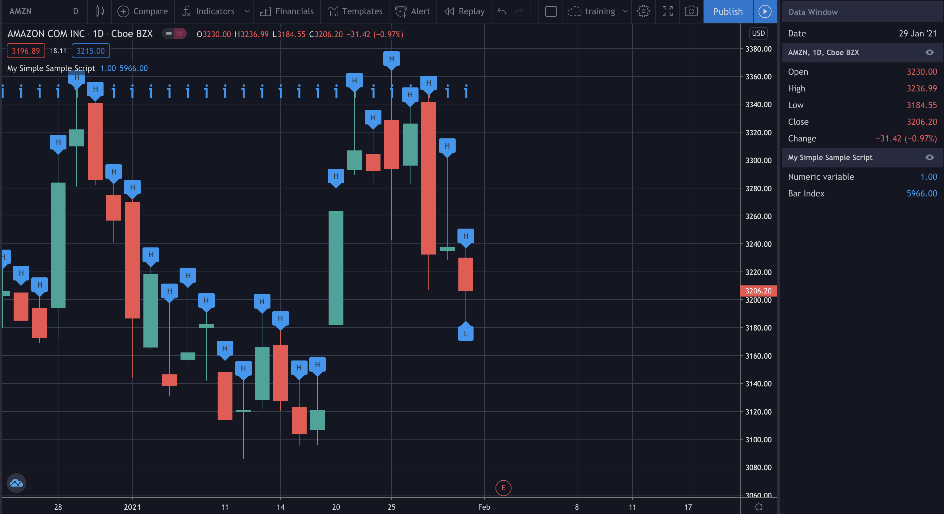
It is not possible to use
plotchar method on Data Window with a string value
plotchar and label.new methods in a function
plotchar method in a local scope like also a for loop
Arrays
Pine arrays are one-dimensional. All elements of an array are of the same type, which can be int, float, bool or color, always of series form.
// initialization of a vector
my_numeric_array = array.new_float(0)
for i = 1 to 6
array.push(my_numeric_array, i)
if barstate.islast // print
label.new(bar_index, high, "my_numeric_array:\n" + tostring(my_numeric_array), style = label.style_label_down, size = size.large)
my_string_array = array.new_string(1, "hello")
array.concat(my_string_array, array.new_string(1, "world"))
array.concat(my_string_array, array.new_string(1, "!"))
if barstate.islast // print
label.new(bar_index, low, "my_string_array: " + array.get(my_string_array, 0), style = label.style_label_up, size = size.large)
my_logic_array = array.new_bool(0)
array.push(my_logic_array, 0)
array.push(my_logic_array, 1)
// operations with arrays
sum = array.sum(my_numeric_array)
mean = array.avg(my_numeric_array)
median = array.median(my_numeric_array)
plotchar(sum, "sum", "")
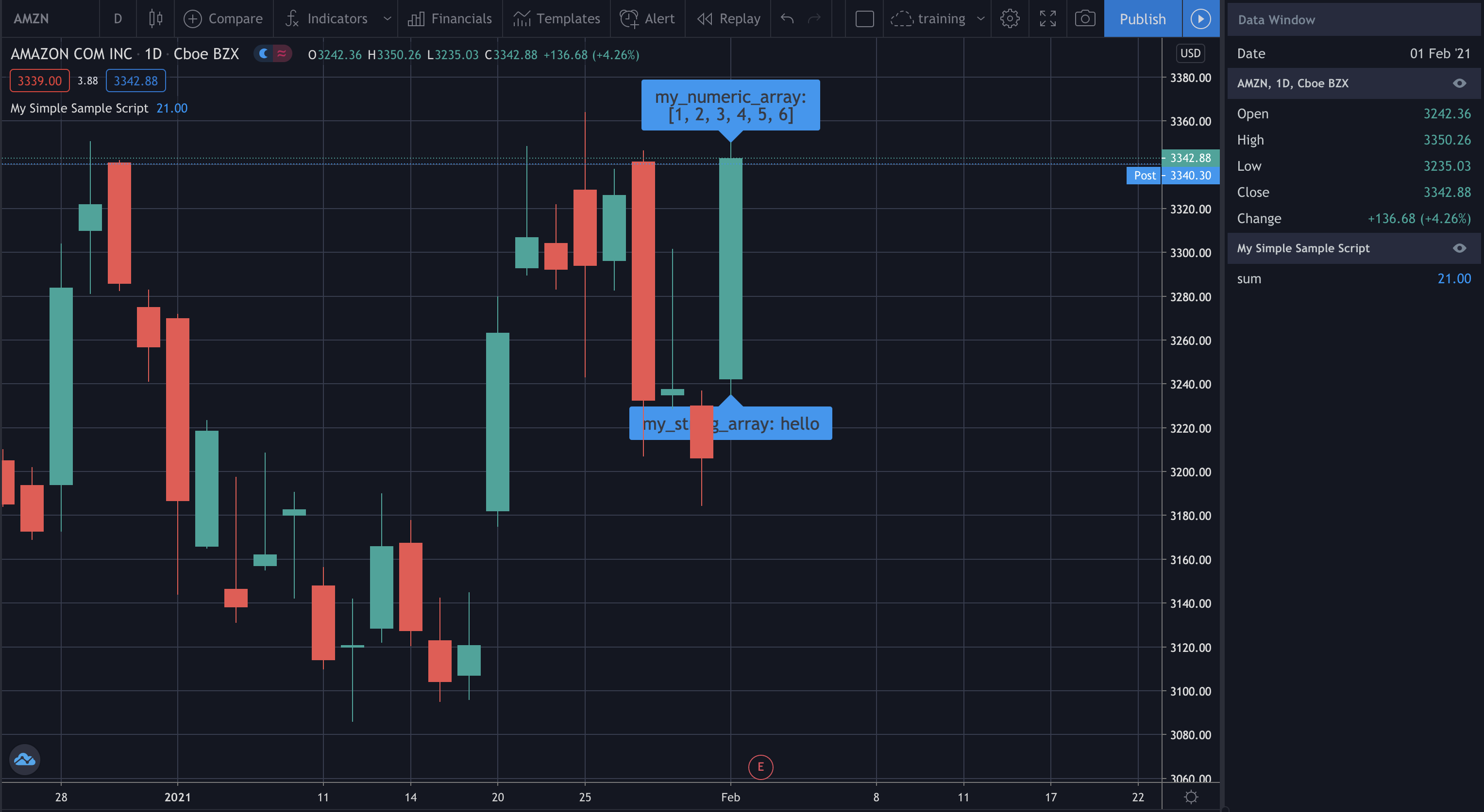
Weighted average
performance = array.new_float(0)
array.push(performance, 3)
array.push(performance, 7)
array.push(performance,11)
weight = array.new_float(0)
array.push(weight, .3)
array.push(weight, .4)
array.push(weight, .3)
weighted_average = array.get(performance, 0) * array.get(weight, 0) + array.get(performance, 1) * array.get(weight, 1) + array.get(performance, 2) * array.get(weight, 2)
plotchar(weighted_average, "weighted_average", "")
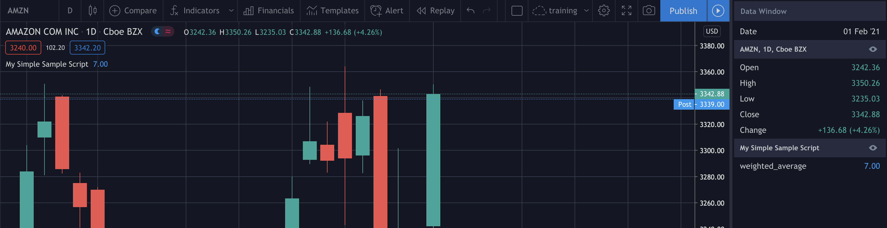
Functions
The functions could return something or not (see the docs for details). The first function named f_print, it returns nothing, only prints on the chart.
// prints on last bar, in the chart space
f_print(_text) =>
// Create label on the first bar.
var _label = label.new(bar_index, na, _text, xloc.bar_index, yloc.price, color(na), label.style_none, color.gray, size.large, text.align_left)
// On next bars, update the label's x and y position, and the text it displays.
label.set_xy(_label, bar_index, highest(10)[1])
label.set_text(_label, _text)
f_print("My details:\nHigh = " + tostring(high))
f_print(my_string_variable + "ello world!\n\n\n")
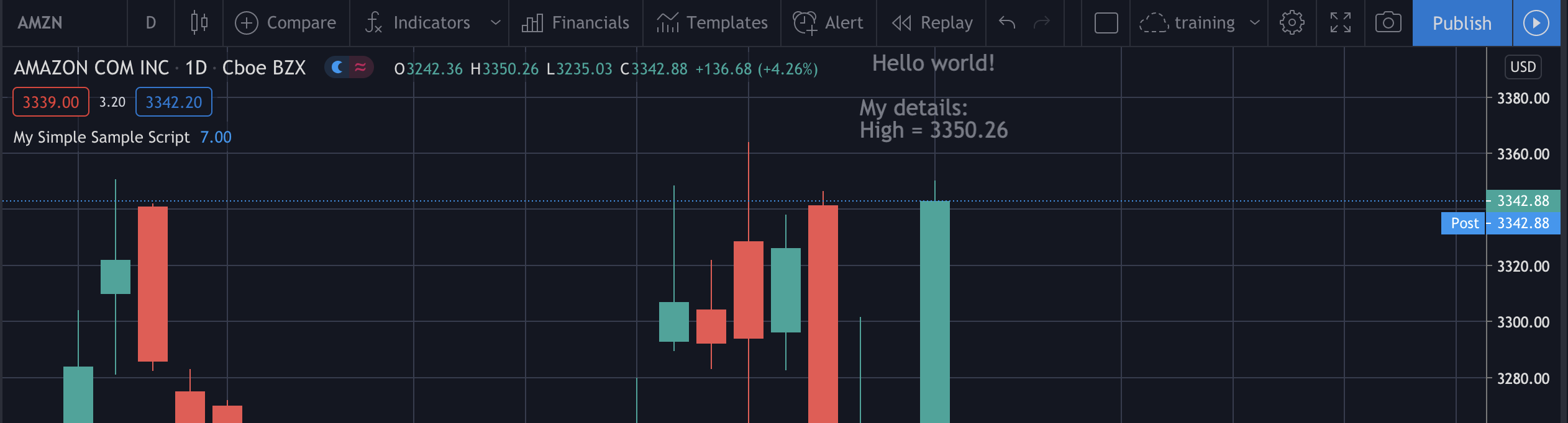
The second function named multiply_performance_weight, it returns an array.
// portfolio performance
company = array.new_string(1, "AAPL")
array.concat(company, array.new_string(1, "NFLX"))
array.concat(company, array.new_string(1, "AMZN"))
multiply_performance_weight(_performance, _weight) =>
_performance_weight = array.new_float(0)
for i = 0 to array.size(_performance) - 1
_one_of_performance_weight = array.get(_performance, i) * array.get(_weight, i)
array.push(_performance_weight, _one_of_performance_weight)
_performance_weight // return the array
And inner a for loop is not possible to use plotchar method, but only label.new method.
performance_weight = multiply_performance_weight(performance, weight)
weighted_average2 = array.sum(performance_weight)
for i = 0 to array.size(performance) - 1
if barstate.islast // print
label.new(bar_index, close, array.get(company, i) + ": " + tostring(array.get(performance_weight, i)), style = label.style_label_up, size = size.large)
plotchar(weighted_average2, "portfolio", "") // Cannot use 'plotchar' in local scope.
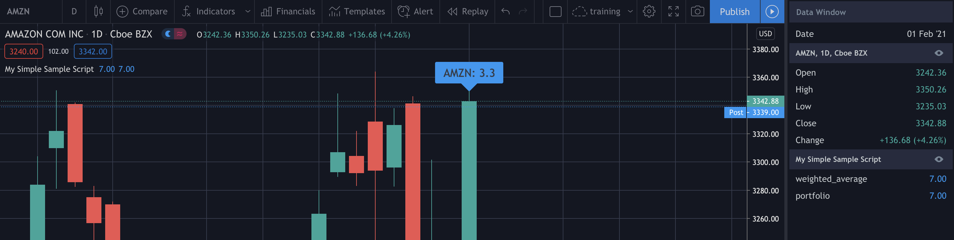
Historical data
Tradingview displays directly the data in the main chart panel, and you can see the all data moving the main chart back.
So, this step is not necessary for using the Pine script language because it is already integrated.
The unique limit is that you can only use the assets present in Tradingview and its partners features.
Graphics
This is a sample for drawing objects with Pine. There are 2 principal methods for drawing, you can draw on
Lines
//@version=4
study("My Simple Sample Script", "", true) // the main chart
You can use the arrays pre loaded for you, like close (values of the closes), and modify them loading only the values that you want
// monthly points - the first Monday of each month
custom = array.new_float(1)
if dayofmonth <= 7 and dayofweek == dayofweek.monday
array.set(custom, 0, close)
else
array.set(custom, 0, na)
customPreviousClose = array.get(custom, 0)[1]
plot(customPreviousClose, "customPreviousClose", color.yellow, 6, plot.style_circles)
plot(customPreviousClose, "customPreviousClose", color.yellow, 6, plot.style_line, transp = 50)
And you can add many many indicators in a few code lines
// moving average
sma25 = sma(close, 25)
ema25 = ema(close, 25)
plot(sma25, "sma 25", color.orange, 2)
plot(ema25, "ema 25", color.red, 2)
// bollinger bands
ma = sma25
dev = 2 * stdev(close, 25)
upper = ma + dev
lower = ma - dev
p1 = plot(upper, color=color.green, linewidth=1, style=plot.style_circles)
p2 = plot(lower, color=color.green, linewidth=1, style=plot.style_circles)
fill(p1, p2)
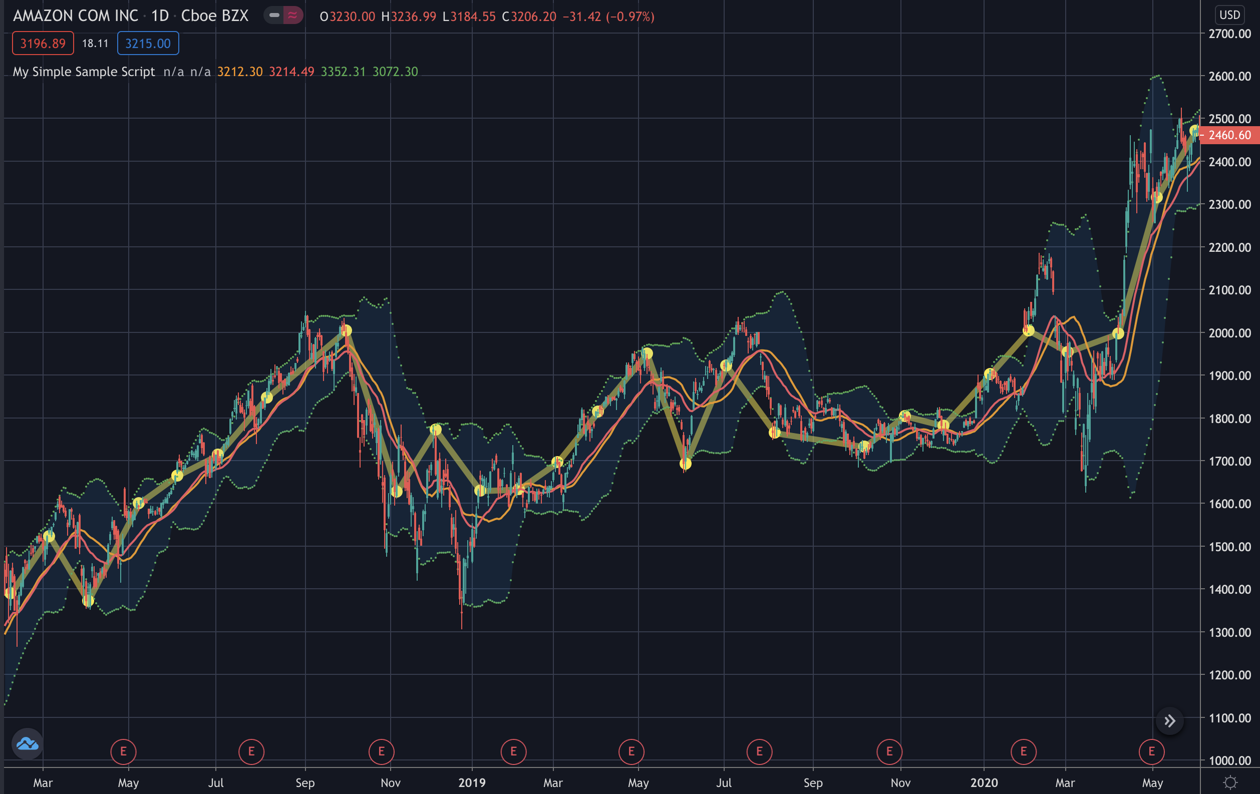
It is possible to draw line from one point to another point, by bar_index or time
// line by index
i = line.new(bar_index, high, bar_index[10], low[10], width = 4)
line.delete(i[1])
// line by time
t = line.new(time, high, time[10], low[10], xloc.bar_time, width = 4)
line.delete(t[1])
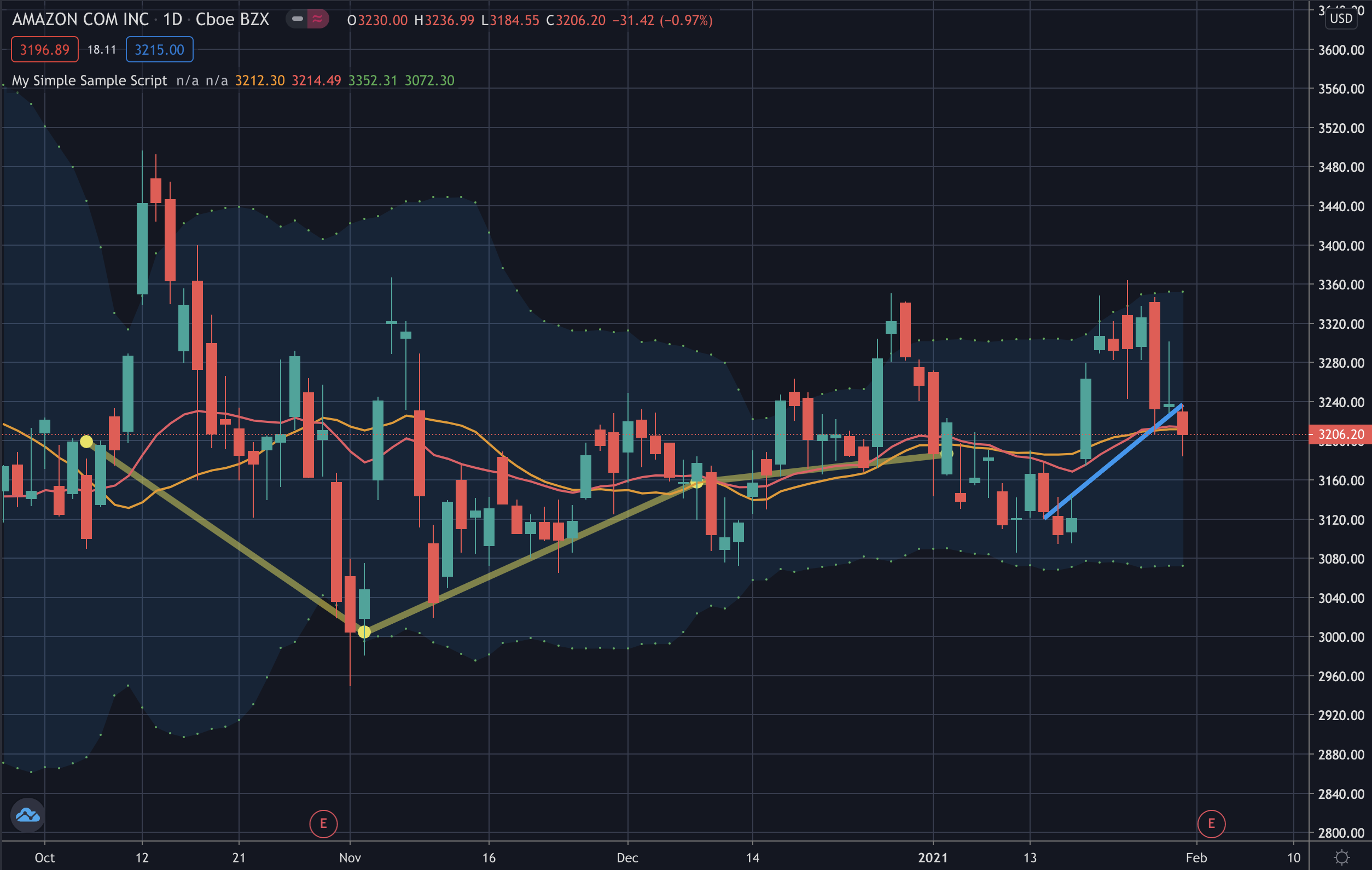
Columns
It is possible to simulate Volume indicator on the main chart with specific parameters
on the study method
adding a workaround that it is the plot of high line
//@version=4
study("My Simple Volume Script", "", true, format.volume, 0, scale.none)
//Get volume for current bar and multiply with vwap
vInverse = volume * vwap
plot(series=vInverse, title="Volume", style=plot.style_columns, color=close >= open ? color.green : color.red, transp=50)
//Plot high line to scale down the columns
highLine = input(1000, "High Line", minval = 2, step = 100)
limit = highest(vInverse, highLine)
scaleFactor = 100 / input(20, "% of vertical space used", step = 10, maxval = 100)
plot(limit * scaleFactor, "Historical High", color.black)
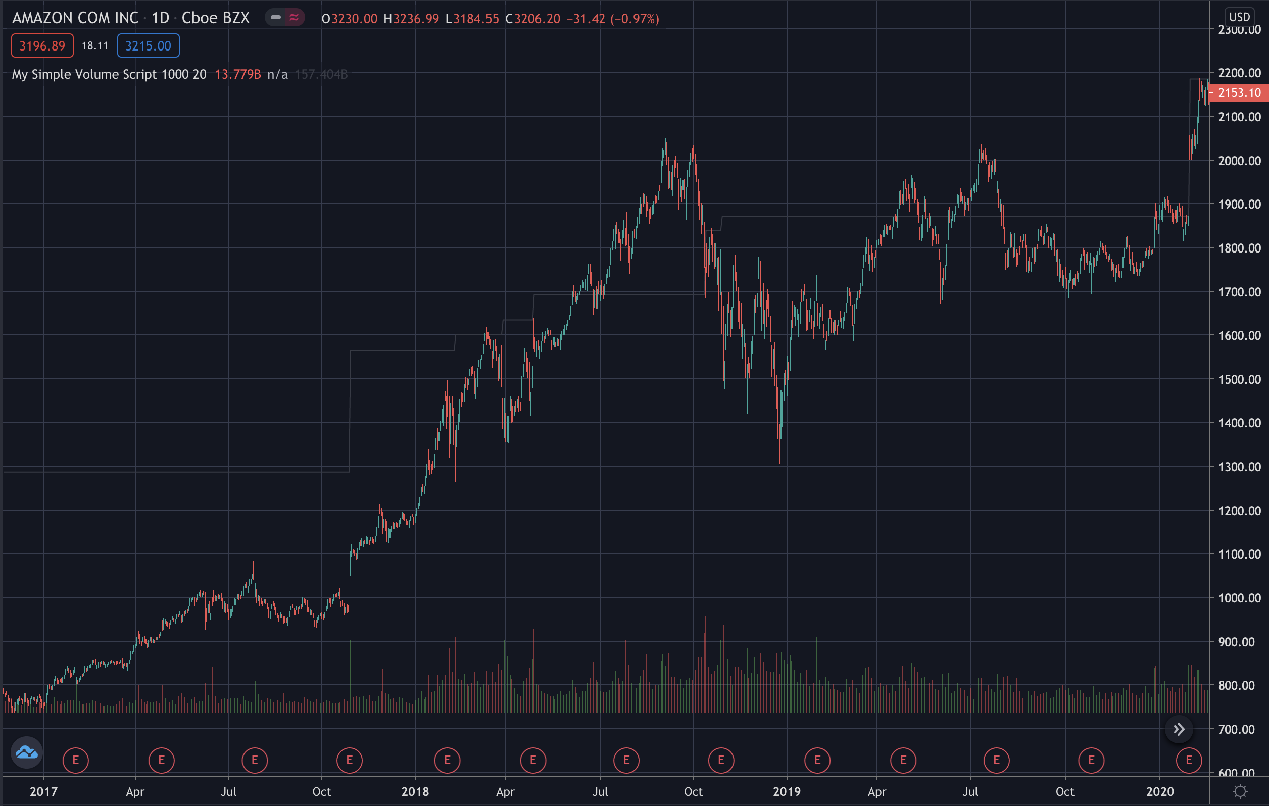
And you can also add SMA indicator over the Volume indicator
//Make the moving average user configurable
showMA = input(true)
plot(showMA ? sma(vInverse,20) : na, title="SMA", style=plot.style_area, color=color.white, transp=80)
The second script has also some inputs that you can manage the values by Settings symbol > Input.
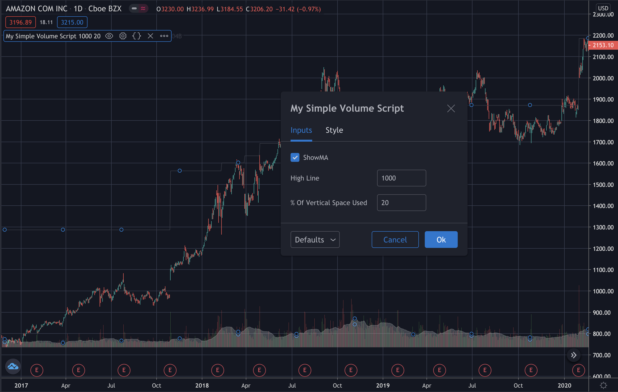
And you can change all colors by Settings symbol > Style.
Points
There are many ready-made methods for you like pivot points.
//@version=4
study("My Simple Pivot Script", "", true)
In that sample you can decide if which plots show by input methods.
legs = input(14)
showPivotHigh = input(true)
showPivotLow = input(true)
And it is used a function, for reusing the code in two points.
pivot_points(pi, legs) =>
newPi = not na(pi)
var float ci = na
if newPi
ci := close[legs]
[pi, newPi, ci]
[pHi, newPHi, cHi] = pivot_points(pivothigh(close, legs, legs), legs)
plot(showPivotHigh ? cHi : na, "", newPHi ? na : color.fuchsia, offset = - legs)
plotchar(showPivotHigh ? pHi : na, "pHi", "▼", location.top, color.fuchsia, offset = - legs)
[pLi, newPLi, cLi] = pivot_points(pivotlow(close, legs, legs), legs)
plot(showPivotLow ? cLi: na, "", newPLi ? na : color.orange, offset = - legs)
plotchar(showPivotLow ? pLi: na, "pLi", "▲", location.bottom, color.orange, offset = - legs)
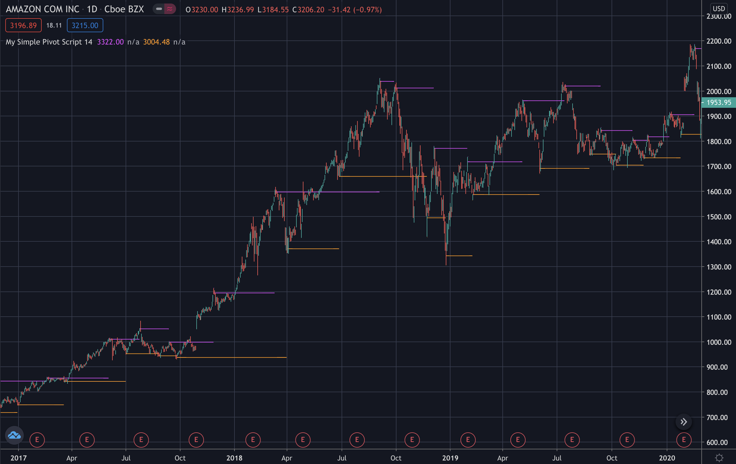
Strategies
You can initilize a strategy by Pine language.
Tradingview has a tab named Strategy Tester near the tab named Pine Editor that it has been created for backtesting your Pine scripts.
How to load indicators on your strategy
When you want to test your strategy on Tradingview, you have to start your Pine script with the method strategy.
//@version=4
strategy("My Simple Strategy Script", "", true) // in the main chart
And then, it is the same for loading your indicators.
A script runs either in overlay=true mode on the chart, in which case it cannot direct plots elsewhere, or in a separate pane when overlay=false (the default).
But there is a workaround for having some plots in the main chart and others in another chart. You can use Settings > Style for flagging who see where you want. So you can also add this code,
// initialization
legs = input(20)
// moving averages
sma20 = sma(close, legs)
plot(sma20, "sma 20", color.blue, 2)
plot(sma(close, 50), "sma 50", color.orange, 2)
// bollinger bands
dev = 2 * stdev(close, legs)
upper = sma20 + dev
lower = sma20 - dev
p1 = plot(upper, title="BB upper", color=color.green, linewidth=1, style=plot.style_circles)
p2 = plot(lower, title="BB lower", color=color.green, linewidth=1, style=plot.style_circles)
fill(p1, p2)
// volume
plot(volume * vwap, title="Volume", style=plot.style_columns, color=close >= open ? color.green : color.red, transp=50)
// rsi
plot(rsi(close, legs), title="RSI", color=color.purple)
h0 = hline(70)
h1 = hline(50)
fill(h0, h1, color=color.purple, transp=75)
Add the chart on the main chart with the header
//@version=4
strategy("My Simple Strategy Script", "", true) // in the main chart
Add the chart on another chart with the header
//@version=4
strategy("My Simple Strategy Script") // a chart space dedicated
And then you can use the Settings for splitting the plots between the main chart and others.
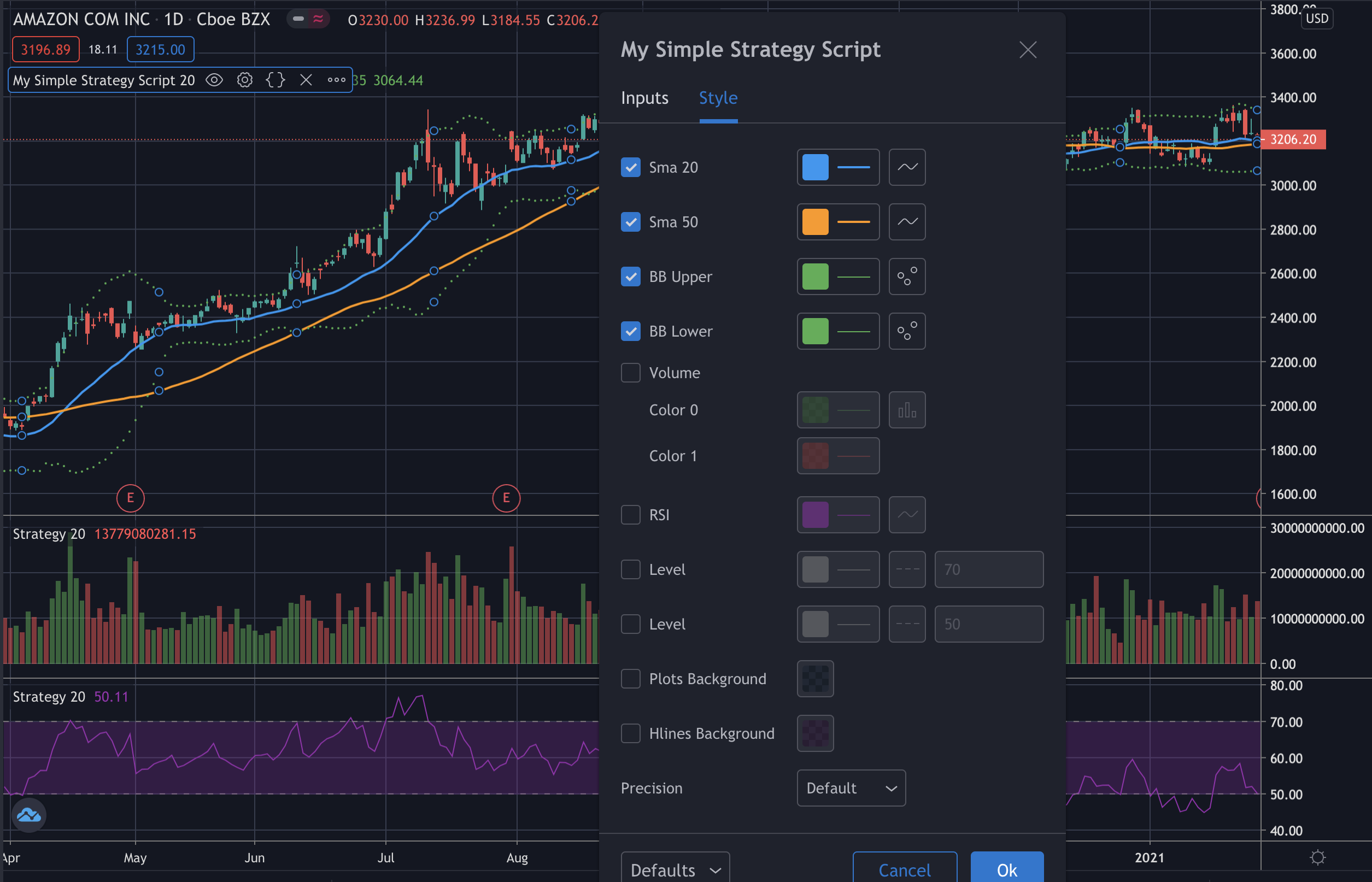
Instead, for the line method it is necessary to use an input and conditions for splitting the lines between the main chart and another. You can use Settings > Input for flagging who see where you want in order of the conditions.
In the code below is used the variable named showLineRSI for the visualization of the lines on RSI chart or the main chart.
// initialization
showLineRSI = input(true)
var bar_time1 = 0
var bar_time2 = 0
var float bar_high1 = 0
var float bar_high2 = 0
var float bar_rsi1 = 0
var float bar_rsi2 = 0
_rsi = rsi(close, 20)
if time == timestamp(2020, 04, 16, 09, 30)
bar_high1 := high
bar_time1 := time
bar_rsi1 := _rsi
if time == timestamp(2020, 05, 21, 09, 30)
bar_high2 := high
bar_time2 := time
bar_rsi2 := _rsi
// rsi line
plot(bar_rsi1 == 0 or bar_rsi2 != 0 ? na : _rsi, title="RSI of trend", color=color.orange, linewidth=2)
plot(rsi(close, 20), title="RSI", color=color.purple)
h0 = hline(70)
h1 = hline(50)
fill(h0, h1, color=color.purple, transp=75)
// rsi trend line
if bar_rsi1 != 0 and bar_rsi2 != 0 and showLineRSI
line.new(bar_time2, bar_rsi2, bar_time1, bar_rsi1, xloc.bar_time, width = 4)
bar_rsi1 := 0
bar_rsi2 := 0
// high line
plot(bar_high1 == 0 or bar_high2 != 0 ? na : high, title="High line", color=color.orange, linewidth=6)
// high trend line
if bar_high1 != 0 and bar_high2 != 0 and showLineRSI != true
line.new(bar_time2, bar_high2, bar_time1, bar_high1, xloc.bar_time, width = 4)
bar_high1 := 0
bar_high2 := 0
And then you can use the Settings and,
Style, for splitting the plots between the main chart and others
Input, for splitting the lines between the main chart and others
In the main chart, for selecting the plots, you can use Settings > Style
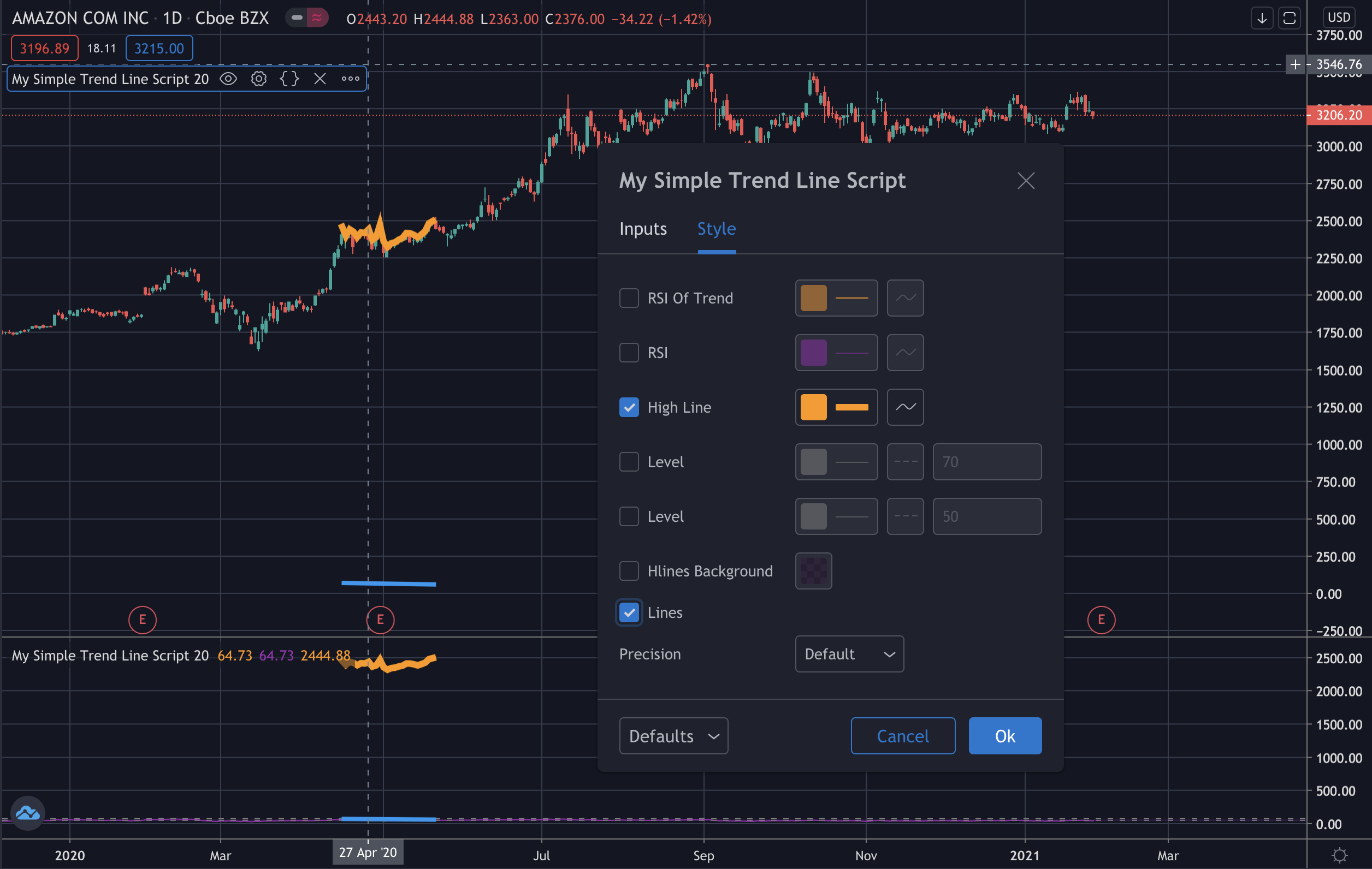
And Settings > Input, for showing the line on the main chart
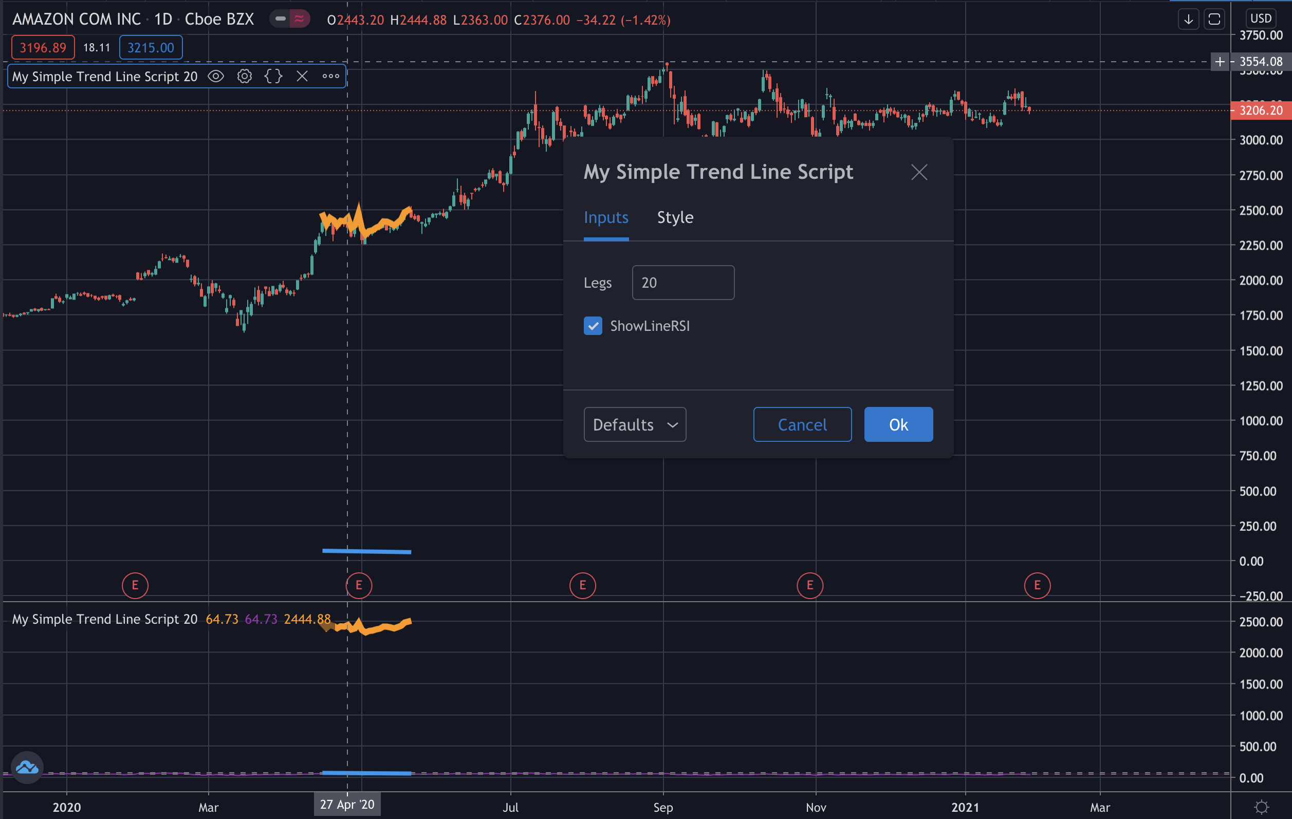
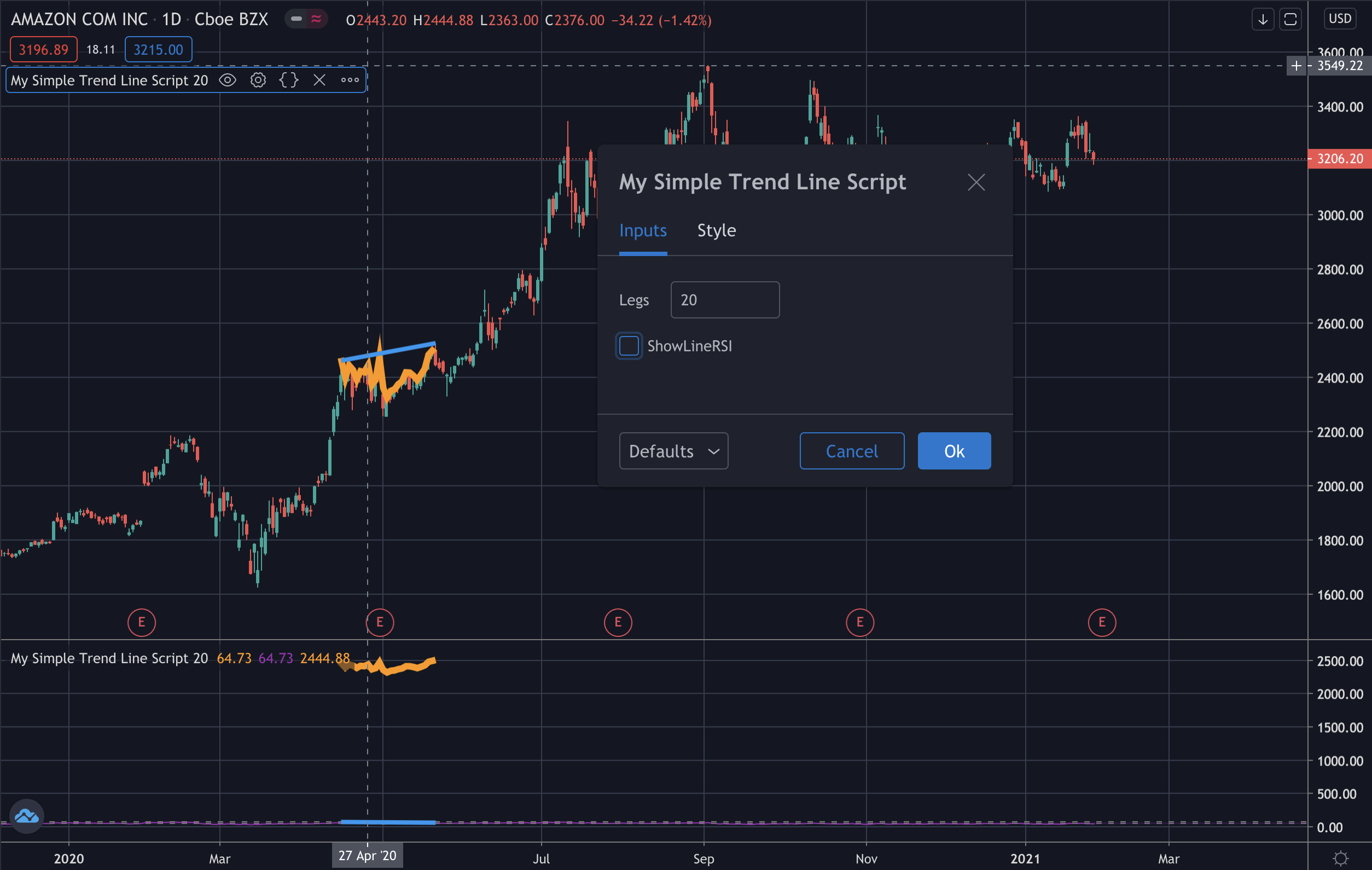
Then, in the other chart, for selecting the plots, you can use Settings > Style
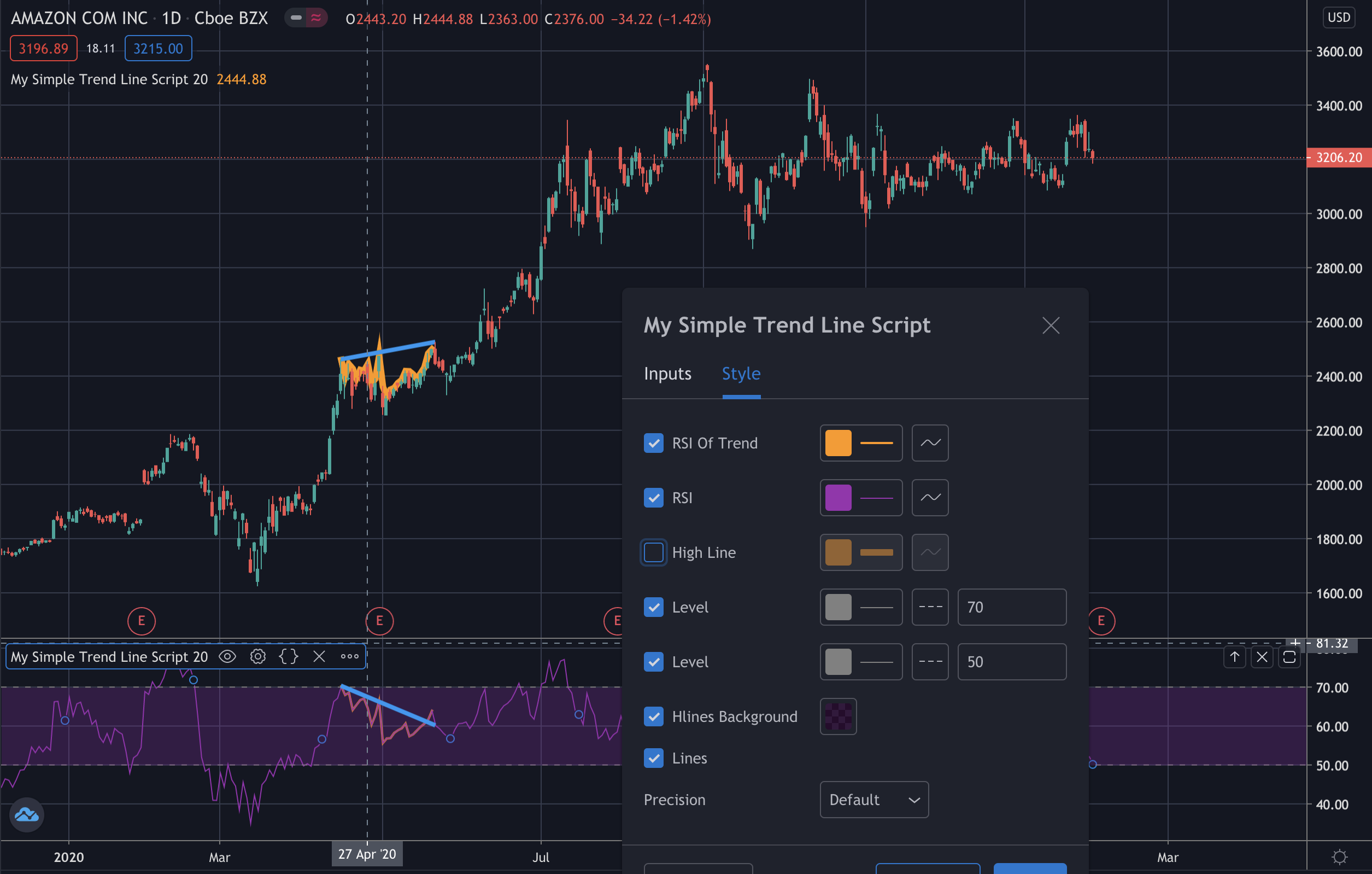
How to load signals on your strategy
The best practice is to prepare one variable for each signal that you want to use on your strategy. The strategy below use the moving averages that they are SMA and EMA. You can use one or the other.
Disclaimer
The strategies below are some simple samples for having an idea how to use the libraries: those strategies are for the educational purpose only. All investments and trading in the stock market involve risk: any decisions related to buying/selling of stocks or other financial instruments should only be made after a thorough research, backtesting, running in demo and seeking a professional assistance if required.
Moving Average Crossover Strategy - Sample 1
when the price value crosses the MA value from below, it will close any existing short position and go long (buy) one unit of the asset
when the price value crosses the MA value from above, it will close any existing long position and go short (sell) one unit of the asset
Reference: https://www.learndatasci.com/tutorials/python-finance-part-3-moving-average-trading-strategy/
//@version=4
//strategy("My Simple Strategy Script - sample 1") // a chart space dedicated
strategy("My Simple Strategy Script - sample 1", "", true) // in the main chart
legs = input(20)
//ma = sma(close, legs)
ma = ema(close, legs)
plot(ma, "Ma", color.orange, 2)
dev = 2 * stdev(close, legs)
upper = ma + dev
lower = ma - dev
p1 = plot(upper, title="BB upper", color=color.green, linewidth=1, style=plot.style_circles)
p2 = plot(lower, title="BB lower", color=color.green, linewidth=1, style=plot.style_circles)
fill(p1, p2)
// Taking the difference between the prices and the MA timeseries
price_ma_diff = close - ma
// Taking the sign of the difference to determine whether the price or the EMA is greater
position = price_ma_diff - price_ma_diff[1]
buyEntry = position >= 2 ? price_ma_diff : na
sellEntry = position <= -2 ? price_ma_diff : na
if (buyEntry)
// strategy.entry("MaLE", strategy.long, stop=lower, oca_name="Ma", oca_type=strategy.oca.cancel, comment="MaLE")
strategy.entry("MaLE", strategy.long, oca_name="Ma", oca_type=strategy.oca.cancel, comment="MaLE")
else
strategy.cancel(id="MaLE")
if (sellEntry)
// strategy.entry("MaSE", strategy.short, stop=upper, oca_name="Ma", oca_type=strategy.oca.cancel, comment="MaSE")
strategy.entry("MaSE", strategy.short, oca_name="Ma", oca_type=strategy.oca.cancel, comment="MaSE")
else
strategy.cancel(id="MaSE")
plot(strategy.equity, title="Equity", color=color.red, linewidth=2, style=plot.style_areabr)
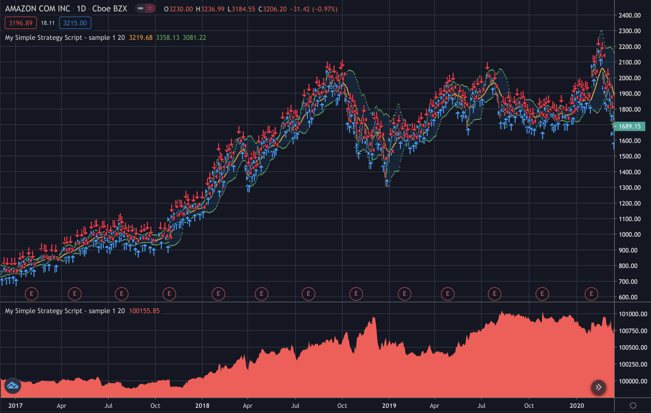
When you Add to Chart your strategy, the Strategy Tester tab will contain the results of your backtesting:
an Overview of the main parameters like Net Profit and Drawdown
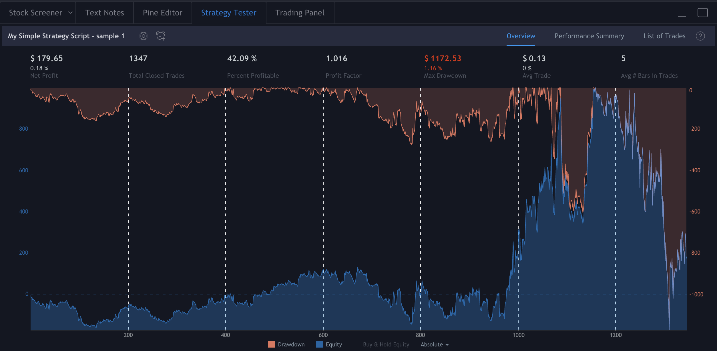
the Performance Summary with all important parameters for defining if your backtesting is good or not
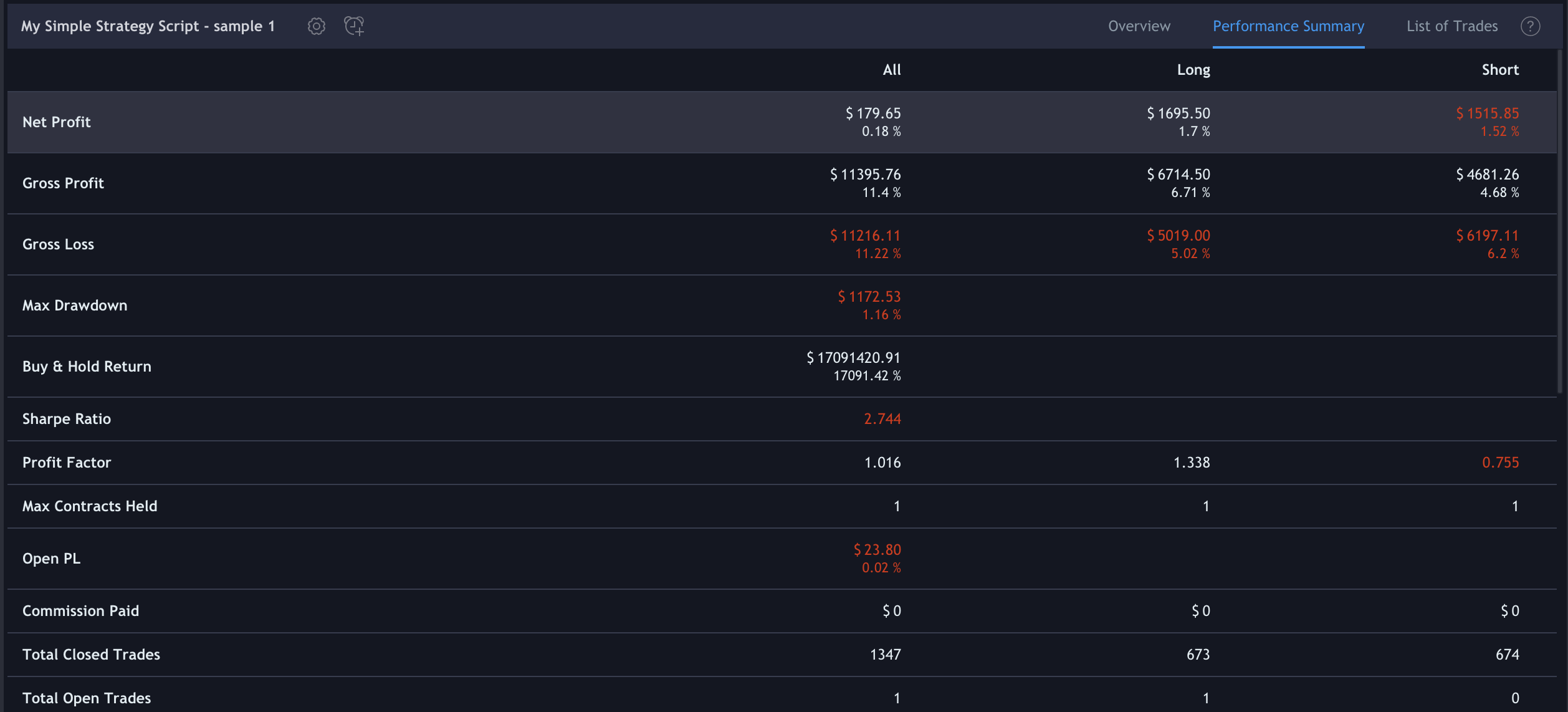
the List of Trades with the details of each trade like Date, Price and Profit
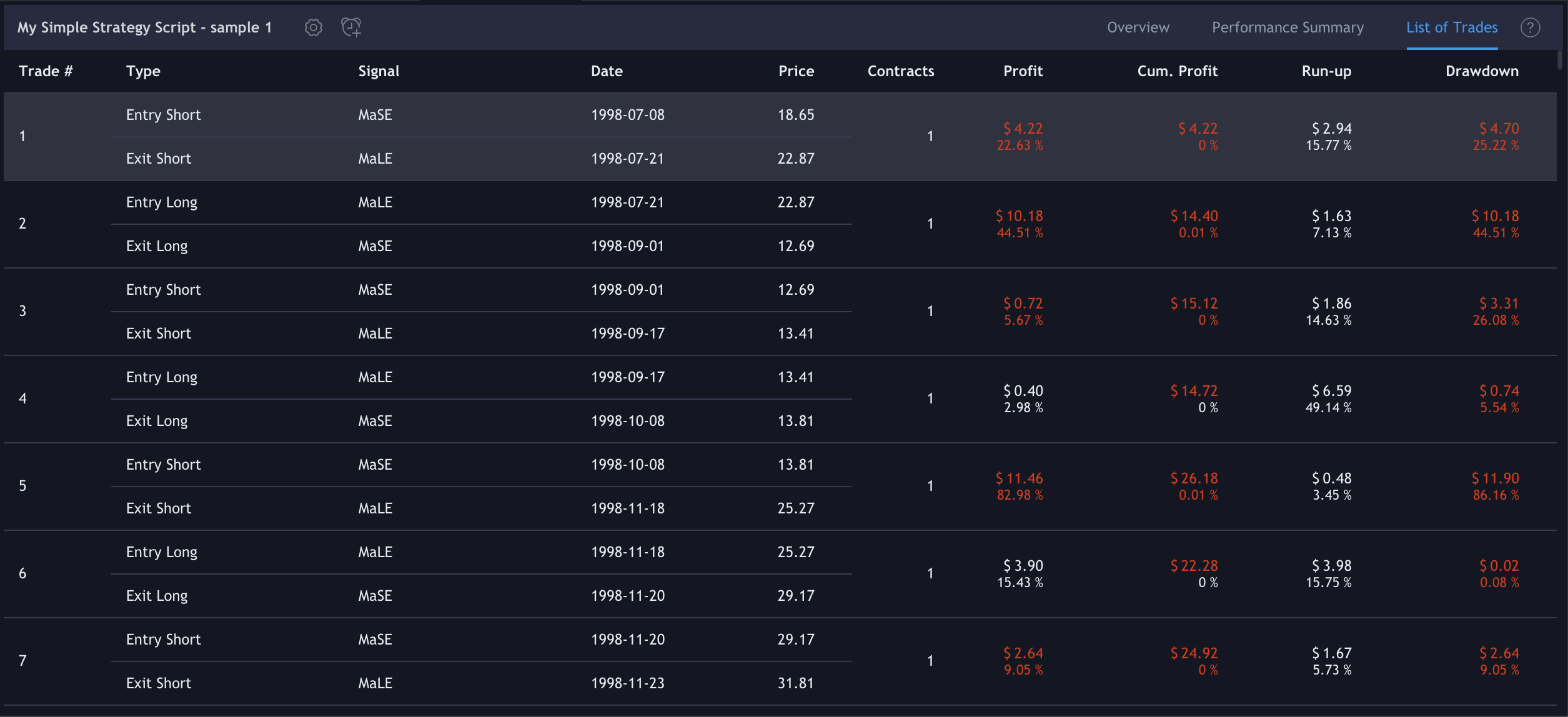
Moving Average Crossover Strategy - Sample 2
when the short term moving average crosses above the long term moving average, this indicates a buy signal
when the short term moving average crosses below the long term moving average, it may be a good moment to sell
//@version=4
//strategy("My Simple Strategy Script - sample 2") // a chart space dedicated
strategy("My Simple Strategy Script - sample 2", "", true) // in the main chart
ma20 = sma(close, 20)
ma50 = sma(close, 50)
//ma20 = ema(close, 20)
//ma50 = ema(close, 50)
plot(ma20, "Ma20", color.blue, 2)
plot(ma50, "Ma50", color.orange, 2)
buyEntry = crossover(ma20, ma50)
sellEntry = crossunder(ma20, ma50)
if (buyEntry)
strategy.entry("MaLE", strategy.long, oca_name="Ma", oca_type=strategy.oca.cancel, comment="MaLE")
else
strategy.cancel(id="MaLE")
if (sellEntry)
strategy.entry("MaSE", strategy.short, oca_name="Ma", oca_type=strategy.oca.cancel, comment="MaSE")
else
strategy.cancel(id="MaSE")
plot(strategy.equity, title="Equity", color=color.red, linewidth=2, style=plot.style_areabr)
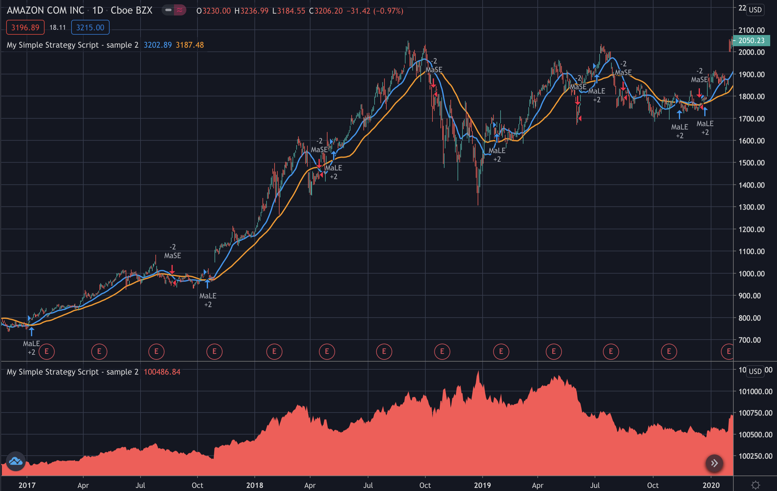
When you Add to Chart your strategy, the Strategy Tester tab will contain the results of your backtesting:
Overview
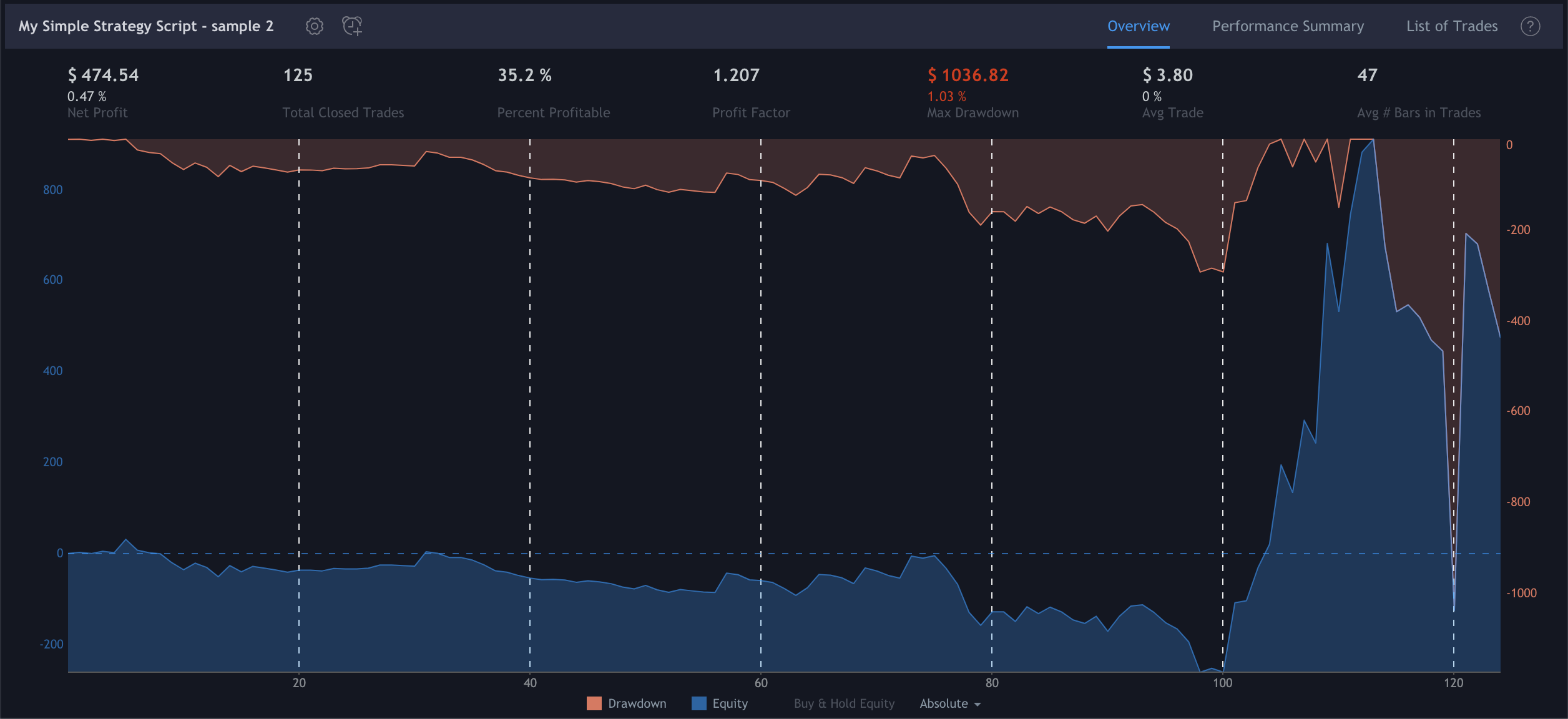
Performance Summary
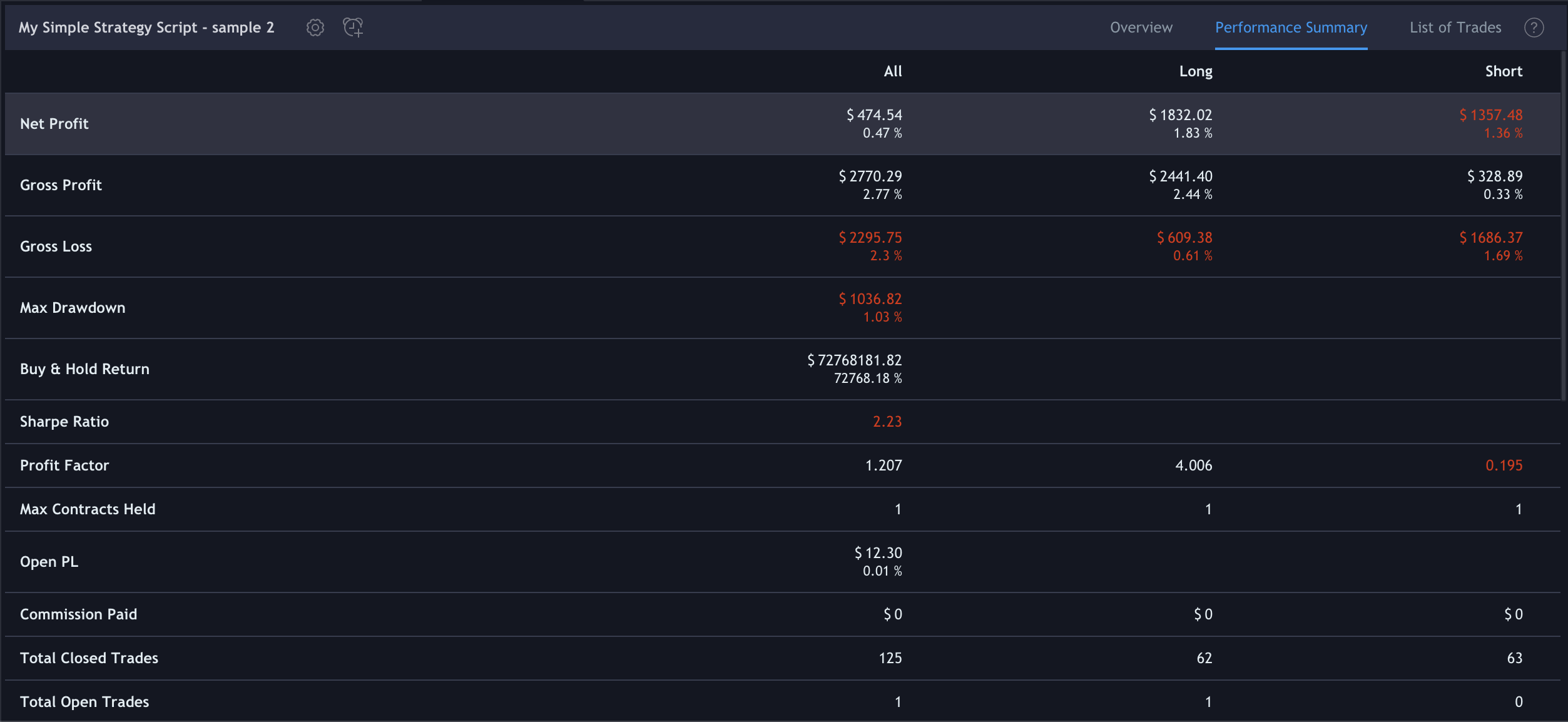
List of Trades
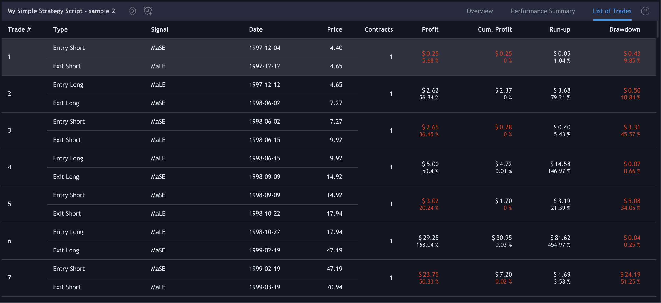
Comparison
The comparison is for evaluating which language or system you could use based on:
maintenance of packages
learning curve / costs
performance
monitoring
In this tutorial, there have been used some languages and systems:
You could know another language or system that it is perfect for your needs. This is only a discussion to highlight key points, bottlenecks and risks.
Maintenance of packages
Learning curve / costs
Performance
Monitoring
Conclusion
Historical data
The samples that you find in this tutorial they use the same data reader: Yahoo Finance API.
This is a tutorial, so it is for educational purpose, and it is not important the results. Each historical data contains some differences among others, so it is very important understanding when using which source.
At the beginning, when you test your code, or learn your instruments, you can also use free historical data. In a perfect system, when your QT system will become your demo and your business, you have to use paid historical data of the trading platform where you will do your demo and your business.
Why do you have to use the same historical data of the trading platform where you will do your demo and your business ?
for avoiding the closing differences or other, that they would completely change the backtesting results
for being prepared for any issue related to those data that will be used for your business (see the Comparison section for details)
Analysis
You cannot make backtesting without defining your trading strategy. And you may not use your trading strategy live without analyze the financial historical data by backtesting.
You can use existing indicators and yours for defining resistence points and signals.
Coming soon.
Best practice
You can use the command line, an IDE or a (Jupyter) notebook for your favorite language or directly a trading platform console, but the rules below do not change: you have to
evaluate your data source and to check (*) that your driver is working properly
test your code by TDD every time that you change it
check (*) your algorithm and its parameters by your backtesting system
evaluate the hosting where you run your QT system and to check (*) that your QT system did not reach its limits
define when your QT system does not have to work
(*) it would be great if each check can run to warn you with a channel you follow about
information of the next release of your driver, your hosting, .. or your trading platform
your algorithm performance
At the beginning, the checks can be executed with a wide cadence, until you find how often each check should be performed according to your expectations. In a perfect system, when your QT system will become your business, the checks will be executed continuously or with a tight cadence.
Coming soon # mql4/index